E16.5 mouse dentate gyrus
library(COTAN)
library(data.table)
library(Matrix)
library(ggrepel)
#> Loading required package: ggplot2
library(latex2exp)
mycolours <- c(A = "#8491B4B2", B = "#E64B35FF")
my_theme = theme(axis.text.x = element_text(size = 14,
angle = 0, hjust = 0.5, vjust = 0.5,
face = "plain", colour = "#3C5488FF"),
axis.text.y = element_text(size = 14,
angle = 0, hjust = 0, vjust = 0.5,
face = "plain", colour = "#3C5488FF"),
axis.title.x = element_text(size = 14,
angle = 0, hjust = 0.5, vjust = 0,
face = "plain", colour = "#3C5488FF"),
axis.title.y = element_text(size = 14,
angle = 90, hjust = 0.5, vjust = 0.5,
face = "plain", colour = "#3C5488FF"))data = as.data.frame(fread(paste(data_dir,
"separation_age/E16.5.csv", sep = "/")))
data = as.data.frame(data)
rownames(data) = data$V1
data = data[, 2:ncol(data)]
data[1:10, 1:10]
#> X10X82_1_CAGAACAAGTTCTG. X10X82_1_TCACTTCTCGCATC.
#> 0610007P14Rik 4 1
#> 0610009B22Rik 1 1
#> 0610009L18Rik 0 0
#> 0610009O20Rik 2 0
#> 0610010F05Rik 0 1
#> 0610010K14Rik 4 0
#> 0610011F06Rik 0 0
#> 0610012D04Rik 0 0
#> 0610012G03Rik 4 1
#> 0610025J13Rik 0 0
#> X10X82_1_TCACTCATATGCTG. X10X82_1_ATGGCTCACGCGGT.
#> 0610007P14Rik 1 1
#> 0610009B22Rik 0 1
#> 0610009L18Rik 0 1
#> 0610009O20Rik 0 0
#> 0610010F05Rik 0 0
#> 0610010K14Rik 0 1
#> 0610011F06Rik 1 1
#> 0610012D04Rik 0 0
#> 0610012G03Rik 3 2
#> 0610025J13Rik 0 0
#> X10X82_1_GGTGCCAACGCACC. X10X82_1_TGAGTTCAAGCCTA.
#> 0610007P14Rik 3 1
#> 0610009B22Rik 1 1
#> 0610009L18Rik 0 0
#> 0610009O20Rik 0 0
#> 0610010F05Rik 0 1
#> 0610010K14Rik 0 0
#> 0610011F06Rik 1 0
#> 0610012D04Rik 0 0
#> 0610012G03Rik 1 2
#> 0610025J13Rik 0 0
#> X10X82_1_CACGATCGCGTTTC. X10X82_1_TATGCGTCCGCTGA.
#> 0610007P14Rik 2 0
#> 0610009B22Rik 0 2
#> 0610009L18Rik 0 0
#> 0610009O20Rik 0 0
#> 0610010F05Rik 1 0
#> 0610010K14Rik 0 0
#> 0610011F06Rik 1 0
#> 0610012D04Rik 0 0
#> 0610012G03Rik 1 3
#> 0610025J13Rik 1 0
#> X10X82_1_TGCTATCGGAAACG. X10X82_1_GTTAGAGCGCTTAT.
#> 0610007P14Rik 2 4
#> 0610009B22Rik 0 0
#> 0610009L18Rik 0 0
#> 0610009O20Rik 0 0
#> 0610010F05Rik 0 0
#> 0610010K14Rik 0 1
#> 0610011F06Rik 0 1
#> 0610012D04Rik 0 0
#> 0610012G03Rik 1 2
#> 0610025J13Rik 0 0Define a directory where the ouput will be stored.
0.1 Analytical pipeline
Initialize the COTAN object with the row count table and the metadata for the experiment.
obj = new("scCOTAN", raw = data)
obj = initRaw(obj, GEO = "GSE104323", sc.method = "10X",
    cond = "mouse dentate gyrus E16.5")
#> [1] "Initializing S4 object"
Now we can start the cleaning. Analysis requires and starts from a matrix of raw UMI counts after removing possible cell doublets or multiplets and low quality or dying cells (with too high mtRNA percentage, easily done with Seurat or other tools).
If we do not want to consider the mitochondrial genes we can remove them before starting the analysis.
genes_to_rem = rownames(obj@raw[grep("^mt",
    rownames(obj@raw)), ])  #genes to remove : mithocondrial
obj@raw = obj@raw[!rownames(obj@raw) %in%
    genes_to_rem, ]
cells_to_rem = colnames(obj@raw[which(colSums(obj@raw) ==
    0)])
obj@raw = obj@raw[, !colnames(obj@raw) %in%
    cells_to_rem]
We want also to define a prefix to identify the sample.
0.2 Data cleaning
First we create the directory to store all information regardin the data cleaning.
if (!file.exists(out_dir)) {
    dir.create(file.path(out_dir))
}

if (!file.exists(paste(out_dir, "cleaning",
    sep = ""))) {
    dir.create(file.path(out_dir, "cleaning"))
}
ttm = clean(obj)
#> [1] "Start estimation mu with linear method"
#> [1] 14131 2285
#> rowname X10X82_1_TACTGAGGCATGGT.
#> 9692 Ptgds 910.01759
#> 7119 Malat1 144.82597
#> 8232 Nnat 56.04377
#> 4619 Ftl1 52.71443
#> 1127 Apoe 44.94599
#> 1404 Atp1a2 43.83621
#> 2343 Cdkn1c 38.84221
#> 2840 Cox4i1 32.73844
#> 2854 Cox8a 32.73844
#> 10515 Rps29 32.18355
#> 3746 Eef1a1 28.29933
#> 10510 Rps27 27.18955
#> 13168 Uqcr11 25.52488
#> 10458 Rpl41 24.41511
#> 10454 Rpl37a 23.30533
obj = ttm$object
ttm$pca.cell.2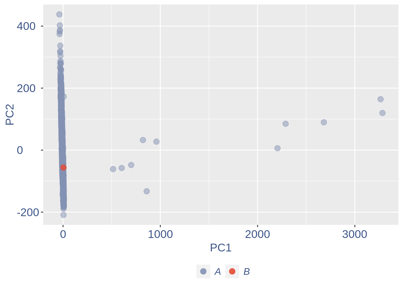
Run this when B cells need to be removed.
pdf(paste(out_dir, "cleaning/", t, "_", n_it,
    "_plots_before_cells_exlusion.pdf", sep = ""))
ttm$pca.cell.2
ggplot(ttm$D, aes(x = n, y = means)) + geom_point() +
    geom_text_repel(data = subset(ttm$D,
        n > (max(ttm$D$n) - 15)), aes(n,
        means, label = rownames(ttm$D[ttm$D$n >
            (max(ttm$D$n) - 15), ])), nudge_y = 0.05,
        nudge_x = 0.05, direction = "x",
        angle = 90, vjust = 0, segment.size = 0.2) +
    ggtitle("B cell group genes mean expression") +
    my_theme + theme(plot.title = element_text(color = "#3C5488FF",
    size = 20, face = "italic", vjust = -5,
    hjust = 0.02))
dev.off()
#> png
#>   2

if (length(ttm$cl1) < length(ttm$cl2)) {
    to_rem = ttm$cl1
} else {
    to_rem = ttm$cl2
}
n_it = n_it + 1
obj@raw = obj@raw[, !colnames(obj@raw) %in%
    to_rem]
# obj@raw = obj@raw[rownames(obj@raw)
# %in% rownames(cells),colnames(obj@raw)
# %in% colnames(cells)]
gc()
#>             used   (Mb) gc trigger   (Mb)  max used   (Mb)
#> Ncells   3706915  198.0    6015681  321.3   6015681  321.3
#> Vcells 231648395 1767.4  347181239 2648.8 347179504 2648.8

ttm = clean(obj)
#> [1] "Start estimation mu with linear method"
#> [1] 14126  2284
#>       rowname X10X82_1_GTTCCGTTCGGGCT. X10X82_1_CGTAAGTAGAAAGG.
#> 12935     Ttr                729.43369               1156.30913
#> 7116   Malat1                140.43227                 68.94445
#> 10455   Rpl41                 60.65046                 85.11661
#> 4618     Ftl1                 38.26270                 31.06756
#> 10502   Rps23                 24.83005                 41.28156
#> 10512   Rps29                 29.30760                 34.04664
#> 10507   Rps27                 23.20185                 28.93965
#> 10489   Rps14                 29.30760                 26.38615
#> 10451  Rpl37a                 25.23710                 33.19548
#> 1792      Bsg                 21.57365                 24.25823
#> 4617     Fth1                 22.79480                 22.13032
#> 10416   Rpl13                 26.45825                 18.30007
#> 3745   Eef1a1                 19.94545                 20.42799
#> 10450   Rpl37                 22.38775                 20.85357
#> 10424  Rpl18a                 21.98070                 19.57682
#>       X10X82_1_CGGATAGCCACGCT.
#> 12935                891.76077
#> 7116                 123.00149
#> 10455                 62.52575
#> 4618                  43.56303
#> 10502                 37.92546
#> 10512                 28.70035
#> 10507                 29.21285
#> 10489                 25.62531
#> 10451                 21.01275
#> 1792                  25.62531
#> 4617                  25.62531
#> 10416                 21.52526
#> 3745                  25.62531
#> 10450                 22.03777
#> 10424                 21.52526
# ttm = clean.sqrt(obj, cells)
obj = ttm$object

ttm$pca.cell.2
Run this only in the last iteration, instead the previous code, when B cells group has not to be removed.
pdf(paste(out_dir, "cleaning/", t, "_", n_it,
    "_plots_before_cells_exlusion.pdf", sep = ""))
ttm$pca.cell.2
ggplot(ttm$D, aes(x = n, y = means)) + geom_point() +
    geom_text_repel(data = subset(ttm$D,
        n > (max(ttm$D$n) - 15)), aes(n,
        means, label = rownames(ttm$D[ttm$D$n >
            (max(ttm$D$n) - 15), ])), nudge_y = 0.05,
        nudge_x = 0.05, direction = "x",
        angle = 90, vjust = 0, segment.size = 0.2) +
    ggtitle(label = "B cell group genes mean expression",
        subtitle = " - B group NOT removed -") +
    my_theme + theme(plot.title = element_text(color = "#3C5488FF",
    size = 20, face = "italic", vjust = -10,
    hjust = 0.02), plot.subtitle = element_text(color = "darkred",
    vjust = -15, hjust = 0.01))

dev.off()
#> png
#>   2
To colour the pca based on nu_j (so the cells’ efficiency).
nu_est = round(obj@nu, digits = 7)

plot.nu <- ggplot(ttm$pca_cells, aes(x = PC1,
    y = PC2, colour = log(nu_est)))

plot.nu = plot.nu + geom_point(size = 1,
    alpha = 0.8) + scale_color_gradient2(low = "#E64B35B2",
    mid = "#4DBBD5B2", high = "#3C5488B2",
    midpoint = log(mean(nu_est)), name = TeX(" $ln (\\nu) $ ")) +
    ggtitle("Cells PCA coloured by cells efficiency") +
    my_theme + theme(plot.title = element_text(color = "#3C5488FF",
    size = 20), legend.title = element_text(color = "#3C5488FF",
    size = 14, face = "italic"), legend.text = element_text(color = "#3C5488FF",
    size = 11), legend.key.width = unit(2,
    "mm"), legend.position = "right")

pdf(paste(out_dir, "cleaning/", t, "_plots_PCA_efficiency_colored.pdf",
    sep = ""))
plot.nu
dev.off()
#> png
#>   2

plot.nu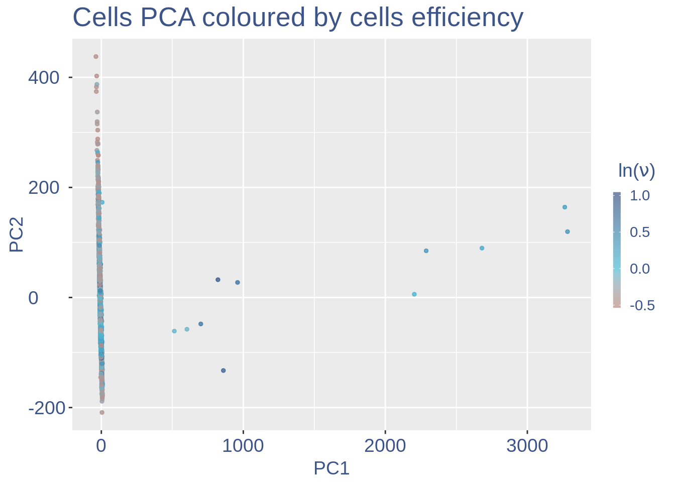
The next part is used to remove the cells with efficiency too low.
nu_df = data.frame(nu = sort(obj@nu), n = c(1:length(obj@nu)))

ggplot(nu_df, aes(x = n, y = nu)) + geom_point(colour = "#8491B4B2",
    size = 1) + my_theme  #+ ylim(0,1) + xlim(0,70)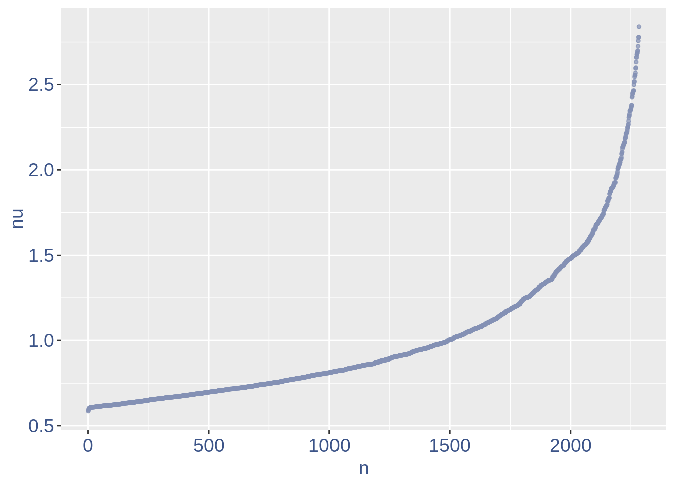
We can zoom on the smallest values and, if we detect a clear elbow, we can decide to remove the cells.
yset = 0.61  #threshold to remove low UDE cells
plot.ude <- ggplot(nu_df, aes(x = n, y = nu)) +
    geom_point(colour = "#8491B4B2", size = 1) +
    my_theme + ylim(0.5, 1) + xlim(0, 800) +
    geom_hline(yintercept = yset, linetype = "dashed",
        color = "darkred") + annotate(geom = "text",
    x = 200, y = 0.5, label = paste("to remove cells with nu < ",
        yset, sep = " "), color = "darkred",
    size = 4.5)


pdf(paste(out_dir, "cleaning/", t, "_plots_efficiency.pdf",
    sep = ""))
plot.ude
dev.off()
#> png
#>   2

plot.ude
We also save the defined threshold in the metadata and re-run the estimation.
obj@meta[(nrow(obj@meta) + 1), 1:2] = c("Threshold low UDE cells:",
    yset)

to_rem = rownames(nu_df[which(nu_df$nu <
    yset), ])

obj@raw = obj@raw[, !colnames(obj@raw) %in%
    to_rem]
Repeat the estimation after the cells are removed.
ttm = clean(obj)
#> [1] "Start estimation mu with linear method"
#> [1] 14119  2259
#>       rowname X10X82_1_GTTCCGTTCGGGCT. X10X82_1_CGTAAGTAGAAAGG.
#> 12928     Ttr                732.65805               1161.42367
#> 7114   Malat1                141.05303                 69.24941
#> 10450   Rpl41                 60.91855                 85.49309
#> 4616     Ftl1                 38.43184                 31.20498
#> 10497   Rps23                 24.93981                 41.46415
#> 10507   Rps29                 29.43715                 34.19724
#> 10502   Rps27                 23.30441                 29.06765
#> 10484   Rps14                 29.43715                 26.50286
#> 10446  Rpl37a                 25.34866                 33.34231
#> 1790      Bsg                 21.66902                 24.36553
#> 4615     Fth1                 22.89556                 22.22820
#> 10411   Rpl13                 26.57521                 18.38101
#> 3743   Eef1a1                 20.03362                 20.51834
#> 10445   Rpl37                 22.48671                 20.94581
#> 10419  Rpl18a                 22.07787                 19.66341
#>       X10X82_1_CGGATAGCCACGCT.
#> 12928                895.71685
#> 7114                 123.54715
#> 10450                 62.80314
#> 4616                  43.75628
#> 10497                 38.09371
#> 10507                 28.82767
#> 10502                 29.34245
#> 10484                 25.73899
#> 10446                 21.10597
#> 1790                  25.73899
#> 4615                  25.73899
#> 10411                 21.62075
#> 3743                  25.73899
#> 10445                 22.13553
#> 10419                 21.62075
obj = ttm$object
ttm$pca.cell.2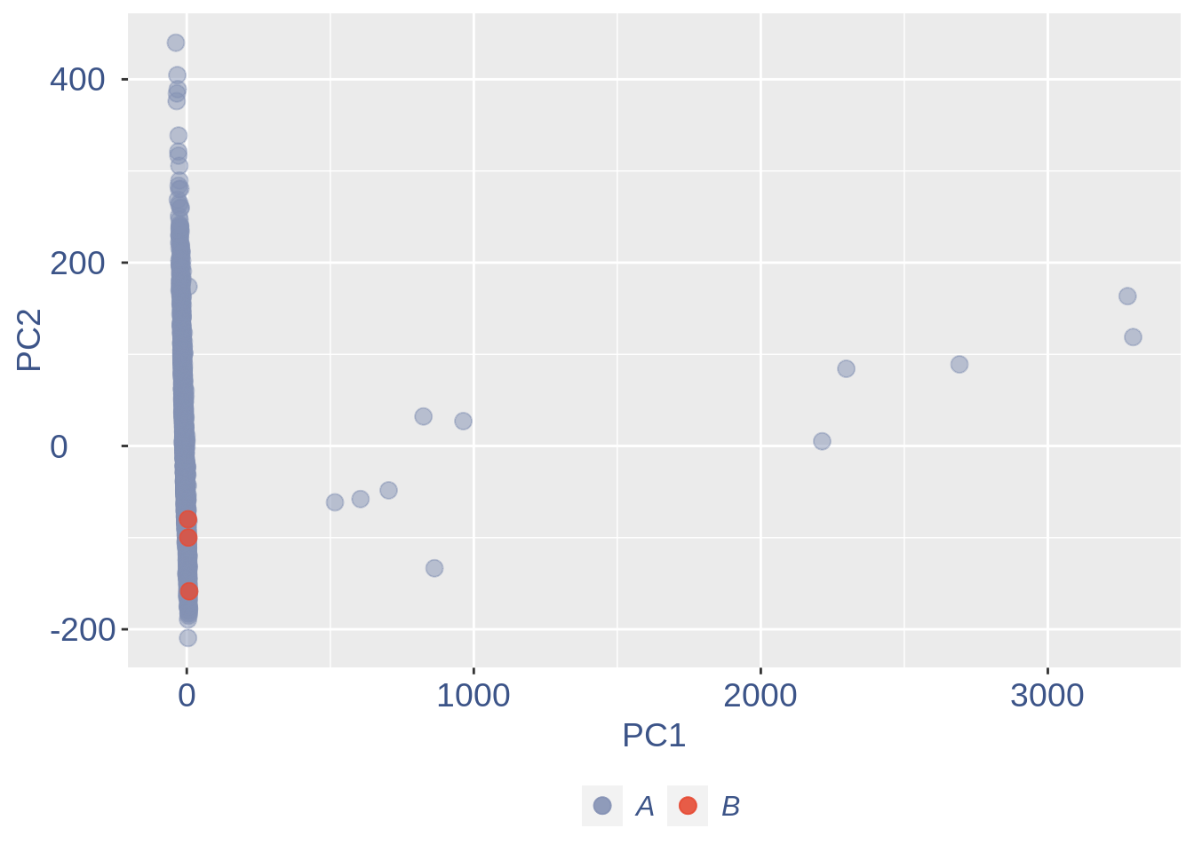
In case we do not want to remove anything, we can run:
pdf(paste(out_dir,"cleaning/",t,"_plots_efficiency.pdf", sep = ""))
ggplot(nu_df, aes(x = n, y=nu)) + geom_point(colour = "#8491B4B2", size=1) +my_theme + #xlim(0,100)+
  annotate(geom="text", x=50, y=0.25, label="nothing to remove ", color="darkred")
dev.off()
#> png
#>   2
Just to check again, we plot the final efficiency coloured PCA.
nu_est = round(obj@nu, digits = 7)
plot.nu <- ggplot(ttm$pca_cells, aes(x = PC1,
    y = PC2, colour = log(nu_est)))
plot.nu = plot.nu + geom_point(size = 2,
    alpha = 0.8) + scale_color_gradient2(low = "#E64B35B2",
    mid = "#4DBBD5B2", high = "#3C5488B2",
    midpoint = log(mean(nu_est)), name = TeX(" $ln (\\nu) $ ")) +
    ggtitle("Cells PCA coloured by cells efficiency: last") +
    my_theme + theme(plot.title = element_text(color = "#3C5488FF",
    size = 20), legend.title = element_text(color = "#3C5488FF",
    size = 14, face = "italic"), legend.text = element_text(color = "#3C5488FF",
    size = 11), legend.key.width = unit(2,
    "mm"), legend.position = "right")

pdf(paste(out_dir, "cleaning/", t, "_plots_PCA_efficiency_colored_FINAL.pdf",
    sep = ""))
plot.nu
dev.off()
#> png
#>   2

plot.nu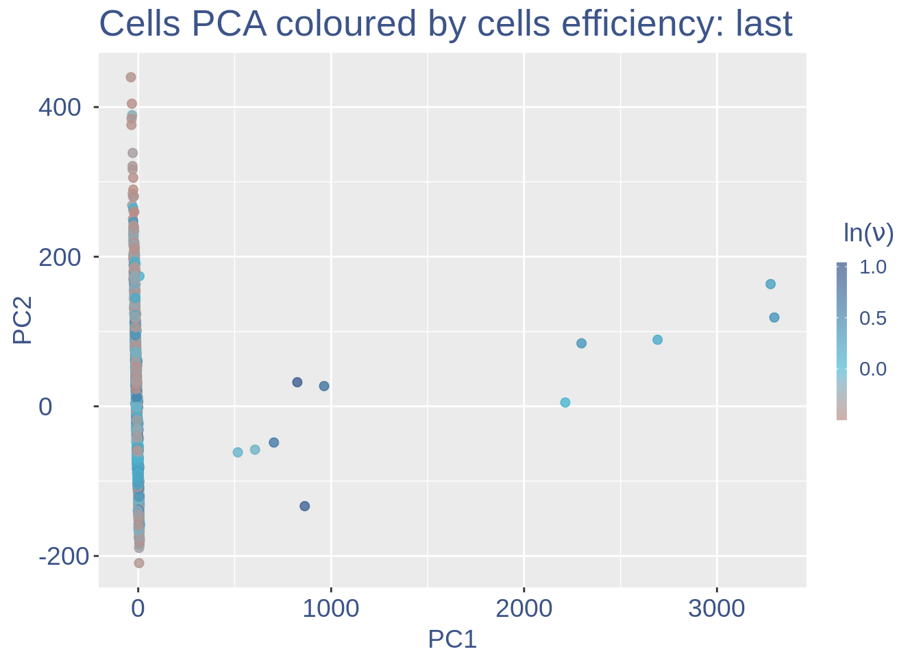
COTAN analysis: in this part all the contingency tables are computed and used to get the statistics (S) To storage efficiency of all the observed tables only the yes_yes is stored.
Note that if will be necessary re-computing the yes-yes table, the yes-yes table should be cancelled before running cotan_analysis.
obj = cotan_analysis(obj)
#> [1] "cotan analysis"
#> [1] "mu estimator creation"
#> [1] "save effective constitutive genes"
#> [1] "start a minimization"
#> [1] "Next gene: Btk number 1810"
#> [1] "Next gene: Eif2d number 3820"
#> [1] "Next gene: Hdhd2 number 5830"
#> [1] "Next gene: Myl12b number 7840"
#> [1] "Next gene: Rab22a number 9850"
#> [1] "Next gene: Swi5 number 11860"
#> [1] "Next gene: Zfp74 number 13870"
#> [1] "Final trance!"
#> [1] "a min: -0.15966796875 | a max 871.25 | negative a %: 23.9152084222507"
COEX evaluation and storing.
saveRDS(obj, file = paste(out_dir, t, ".cotan.RDS",
    sep = ""))

obj = get.coex(obj)
#> [1] "coex dataframe creation"
#> [1] "Generating contingency tables for observed data"
#> [1] "creation of observed yes/yes contingency table"
#> [1] "mu estimator creation"
#> [1] "expected contingency tables creation"
#> [1] "The distance between estimated n of zeros and observed number of zero is 0.0638973580200531 over 14058"
#> [1] "Done"
#> [1] "coex estimation"
#> [1] "Diagonal coex values substituted with 0"

# saving the structure
saveRDS(obj, file = paste(out_dir, t, ".cotan.RDS",
    sep = ""))
Automatic data elaboration (without cleaning)
obj2 = automatic.COTAN.object.creation(df = data,
    GEO = "GSE104323", sc.method = "10X",
    cond = "E16_dent_gy", out_dir = "Data/")
#> [1] "Initializing S4 object"
#> [1] "Condition E16_dent_gy"
#> [1] "n cells 2285"
#> [1] "Start estimation mu with linear method"
#> [1] 14131  2285
#>       rowname X10X82_1_TACTGAGGCATGGT.
#> 9692    Ptgds                910.01759
#> 7119   Malat1                144.82597
#> 8232     Nnat                 56.04377
#> 4619     Ftl1                 52.71443
#> 1127     Apoe                 44.94599
#> 1404   Atp1a2                 43.83621
#> 2343   Cdkn1c                 38.84221
#> 2840   Cox4i1                 32.73844
#> 2854    Cox8a                 32.73844
#> 10515   Rps29                 32.18355
#> 3746   Eef1a1                 28.29933
#> 10510   Rps27                 27.18955
#> 13168  Uqcr11                 25.52488
#> 10458   Rpl41                 24.41511
#> 10454  Rpl37a                 23.30533
#> [1] "Cotan analysis function started"
#> [1] "cotan analysis"
#> [1] "mu estimator creation"
#> [1] "save effective constitutive genes"
#> [1] "start a minimization"
#> [1] "Next gene: Btg1 number 1810"
#> [1] "Next gene: Eif2b3 number 3820"
#> [1] "Next gene: Hddc3 number 5830"
#> [1] "Next gene: Myh2 number 7840"
#> [1] "Next gene: Rab14 number 9850"
#> [1] "Next gene: Suv420h1 number 11860"
#> [1] "Next gene: Zfp706 number 13870"
#> [1] "a min: -0.16796875 | a max 881.25 | negative a %: 23.9800995024876"
#> [1] "Only analysis time 2.71626739501953"
#> [1] "Cotan coex estimation started"
#> [1] "coex dataframe creation"
#> [1] "Generating contingency tables for observed data"
#> [1] "creation of observed yes/yes contingency table"
#> [1] "mu estimator creation"
#> [1] "expected contingency tables creation"
#> [1] "The distance between estimated n of zeros and observed number of zero is 0.0633983950493963 over 14070"
#> [1] "Done"
#> [1] "coex estimation"
#> [1] "Diagonal coex values substituted with 0"
#> [1] "Total time 5.0609365383784"
#> [1] "Only coex time 1.99707407156626"
#> [1] "Saving elaborated data locally at Data/E16_dent_gy.cotan.RDS"
1 Analysis of the elaborated data
In this case the test possible macroscopic differences between cleaned and not cleaned data.
The initial cell number was:
obj@meta
#>                         V1                        V2
#> 1                     GEO:                 GSE104323
#> 2         scRNAseq method:                       10X
#> 3    starting n. of cells:                      2285
#> 4        Condition sample: mouse dentate gyrus E16.5
#> 5 Threshold low UDE cells:                      0.61
While the final number of cells was:
So were removed:
cells
1.1 GDI with cleaning
quant.p = get.GDI(obj)
#> [1] "function to generate GDI dataframe"
#> [1] "Using S"
#> [1] "function to generate S "

head(quant.p)
#>               sum.raw.norm      GDI exp.cells
#> 0610007P14Rik     7.771356 1.757084 61.000443
#> 0610009B22Rik     7.481643 1.433632 52.058433
#> 0610009L18Rik     5.796126 1.570076 13.103143
#> 0610009O20Rik     5.366675 1.915944  8.632138
#> 0610010F05Rik     7.335761 2.961452 44.001771
#> 0610010K14Rik     7.414252 1.500532 49.535193
In the third column of this data frame is reported the percentage of cells expressing the gene.
NPGs = c("Nes", "Vim", "Sox2", "Sox1", "Notch1",
    "Hes1", "Hes5", "Pax6")  #,'Hes3'
PNGs = c("Map2", "Tubb3", "Neurod1", "Nefm",
    "Nefl", "Dcx", "Tbr1")
hk = c("Calm1", "Cox6b1", "Ppia", "Rpl18",
    "Cox7c", "Erh", "H3f3a", "Taf1", "Taf2",
    "Gapdh", "Actb", "Golph3", "Mtmr12",
    "Zfr", "Sub1", "Tars", "Amacr")

text.size = 12

quant.p$highlight = with(quant.p, ifelse(rownames(quant.p) %in%
    NPGs, "NPGs", ifelse(rownames(quant.p) %in%
    hk, "Constitutive", ifelse(rownames(quant.p) %in%
    PNGs, "PNGs", "normal"))))

textdf <- quant.p[rownames(quant.p) %in%
    c(NPGs, hk, PNGs), ]
mycolours <- c(Constitutive = "#00A087FF",
    NPGs = "#E64B35FF", PNGs = "#F39B7FFF",
    normal = "#8491B4B2")
f1 = ggplot(subset(quant.p, highlight ==
    "normal"), aes(x = sum.raw.norm, y = GDI)) +
    geom_point(alpha = 0.1, color = "#8491B4B2",
        size = 2.5)
GDI_plot = f1 + geom_point(data = subset(quant.p,
    highlight != "normal"), aes(x = sum.raw.norm,
    y = GDI, colour = highlight), size = 2.5,
    alpha = 0.8) + geom_hline(yintercept = quantile(quant.p$GDI)[4],
    linetype = "dashed", color = "darkblue") +
    geom_hline(yintercept = quantile(quant.p$GDI)[3],
        linetype = "dashed", color = "darkblue") +
    geom_hline(yintercept = 1.5, linetype = "dotted",
        color = "red", size = 0.5) + scale_color_manual("Status",
    values = mycolours) + scale_fill_manual("Status",
    values = mycolours) + xlab("log normalized counts") +
    ylab("GDI") + geom_label_repel(data = textdf,
    aes(x = sum.raw.norm, y = GDI, label = rownames(textdf),
        fill = highlight), label.size = NA,
    alpha = 0.5, direction = "both", na.rm = TRUE,
    seed = 1234) + geom_label_repel(data = textdf,
    aes(x = sum.raw.norm, y = GDI, label = rownames(textdf)),
    label.size = NA, segment.color = "black",
    segment.size = 0.5, direction = "both",
    alpha = 0.8, na.rm = TRUE, fill = NA,
    seed = 1234) + theme(axis.text.x = element_text(size = text.size,
    angle = 0, hjust = 0.5, vjust = 0.5,
    face = "plain", colour = "#3C5488FF"),
    axis.text.y = element_text(size = text.size,
        angle = 0, hjust = 0, vjust = 0.5,
        face = "plain", colour = "#3C5488FF"),
    axis.title.x = element_text(size = text.size,
        angle = 0, hjust = 0.5, vjust = 0,
        face = "plain", colour = "#3C5488FF"),
    axis.title.y = element_text(size = text.size,
        angle = 90, hjust = 0.5, vjust = 0.5,
        face = "plain", colour = "#3C5488FF"),
    legend.title = element_blank(), legend.text = element_text(color = "#3C5488FF",
        face = "italic"), legend.position = "bottom")  # titl)
legend <- cowplot::get_legend(GDI_plot)
GDI_plot = GDI_plot + theme(legend.position = "none")
GDI_plot
1.2 GDI without cleaning
quant.p = get.GDI(obj2)
#> [1] "function to generate GDI dataframe"
#> [1] "Using S"
#> [1] "function to generate S "

head(quant.p)
#>               sum.raw.norm      GDI exp.cells
#> 0610007P14Rik     7.777981 1.756868 60.831510
#> 0610009B22Rik     7.491839 1.442903 51.903720
#> 0610009L18Rik     5.812074 1.560409 13.129103
#> 0610009O20Rik     5.362669 1.918659  8.533917
#> 0610010F05Rik     7.345695 2.959066 43.938731
#> 0610010K14Rik     7.420519 1.505370 49.409190
In the third column of this data frame is reported the percentage of cells expressing the gene.
NPGs = c("Nes", "Vim", "Sox2", "Sox1", "Notch1",
    "Hes1", "Hes5", "Pax6")  #,'Hes3'
PNGs = c("Map2", "Tubb3", "Neurod1", "Nefm",
    "Nefl", "Dcx", "Tbr1")
hk = c("Calm1", "Cox6b1", "Ppia", "Rpl18",
    "Cox7c", "Erh", "H3f3a", "Taf1", "Taf2",
    "Gapdh", "Actb", "Golph3", "Mtmr12",
    "Zfr", "Sub1", "Tars", "Amacr")

text.size = 12

quant.p$highlight = with(quant.p, ifelse(rownames(quant.p) %in%
    NPGs, "NPGs", ifelse(rownames(quant.p) %in%
    hk, "Constitutive", ifelse(rownames(quant.p) %in%
    PNGs, "PNGs", "normal"))))

textdf <- quant.p[rownames(quant.p) %in%
    c(NPGs, hk, PNGs), ]
mycolours <- c(Constitutive = "#00A087FF",
    NPGs = "#E64B35FF", PNGs = "#F39B7FFF",
    normal = "#8491B4B2")
f1 = ggplot(subset(quant.p, highlight ==
    "normal"), aes(x = sum.raw.norm, y = GDI)) +
    geom_point(alpha = 0.1, color = "#8491B4B2",
        size = 2.5)
GDI_plot = f1 + geom_point(data = subset(quant.p,
    highlight != "normal"), aes(x = sum.raw.norm,
    y = GDI, colour = highlight), size = 2.5,
    alpha = 0.8) + geom_hline(yintercept = quantile(quant.p$GDI)[4],
    linetype = "dashed", color = "darkblue") +
    geom_hline(yintercept = quantile(quant.p$GDI)[3],
        linetype = "dashed", color = "darkblue") +
    geom_hline(yintercept = 1.5, linetype = "dotted",
        color = "red", size = 0.5) + scale_color_manual("Status",
    values = mycolours) + scale_fill_manual("Status",
    values = mycolours) + xlab("log normalized counts") +
    ylab("GDI") + geom_label_repel(data = textdf,
    aes(x = sum.raw.norm, y = GDI, label = rownames(textdf),
        fill = highlight), label.size = NA,
    alpha = 0.5, direction = "both", na.rm = TRUE,
    seed = 1234) + geom_label_repel(data = textdf,
    aes(x = sum.raw.norm, y = GDI, label = rownames(textdf)),
    label.size = NA, segment.color = "black",
    segment.size = 0.5, direction = "both",
    alpha = 0.8, na.rm = TRUE, fill = NA,
    seed = 1234) + theme(axis.text.x = element_text(size = text.size,
    angle = 0, hjust = 0.5, vjust = 0.5,
    face = "plain", colour = "#3C5488FF"),
    axis.text.y = element_text(size = text.size,
        angle = 0, hjust = 0, vjust = 0.5,
        face = "plain", colour = "#3C5488FF"),
    axis.title.x = element_text(size = text.size,
        angle = 0, hjust = 0.5, vjust = 0,
        face = "plain", colour = "#3C5488FF"),
    axis.title.y = element_text(size = text.size,
        angle = 90, hjust = 0.5, vjust = 0.5,
        face = "plain", colour = "#3C5488FF"),
    legend.title = element_blank(), legend.text = element_text(color = "#3C5488FF",
        face = "italic"), legend.position = "bottom")  # titl)
legend <- cowplot::get_legend(GDI_plot)
GDI_plot = GDI_plot + theme(legend.position = "none")
GDI_plot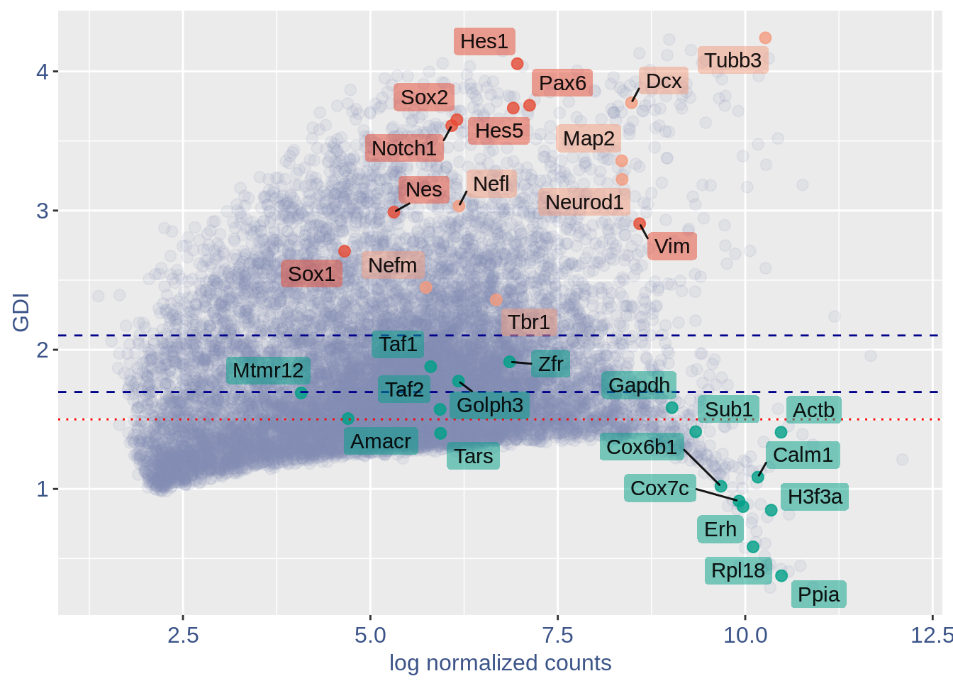
1.3 Heatmaps with cleaning
For the Gene Pair Analysis, we can plot an heatmap with the coex values between two genes sets. To do so we need to define, in a list, the different gene sets (list.genes). Then in the function parameter sets we can decide which sets need to be considered (in the example from 1 to 3). In the condition parameter we should insert an array with each file name prefix to be considered (in the example, the file names is “E15_cortex_clean”).
list.genes = list(Ref.col = PNGs, NPGs = NPGs,
    Const. = hk)

plot_heatmap(df_genes = list.genes, sets = c(1:3),
    conditions = "E16.5_cleaned", dir = "Data/")
#> [1] "plot heatmap"
#> [1] "Loading condition E16.5_cleaned"
#> [1] "Map2"    "Tubb3"   "Neurod1" "Nefm"    "Nefl"    "Dcx"     "Tbr1"
#> [1] "Get p-values on a set of genes on columns on a set of genes on rows"
#> [1] "Using function S"
#> [1] "function to generate S "
#> [1] "Ref.col"
#> [1] "NPGs"
#> [1] "Const."
#> [1] "min coex: -0.0118943380956698 max coex 0.010004681362927"
1.4 Heatmaps without cleaning
list.genes = list(Ref.col = PNGs, NPGs = NPGs,
    Const. = hk)

plot_heatmap(df_genes = list.genes, sets = c(1:3),
    conditions = "E16_dent_gy", dir = "Data/")
#> [1] "plot heatmap"
#> [1] "Loading condition E16_dent_gy"
#> [1] "Map2"    "Tubb3"   "Neurod1" "Nefm"    "Nefl"    "Dcx"     "Tbr1"
#> [1] "Get p-values on a set of genes on columns on a set of genes on rows"
#> [1] "Using function S"
#> [1] "function to generate S "
#> [1] "Ref.col"
#> [1] "NPGs"
#> [1] "Const."
#> [1] "min coex: -0.0118691182192925 max coex 0.0099495109519959"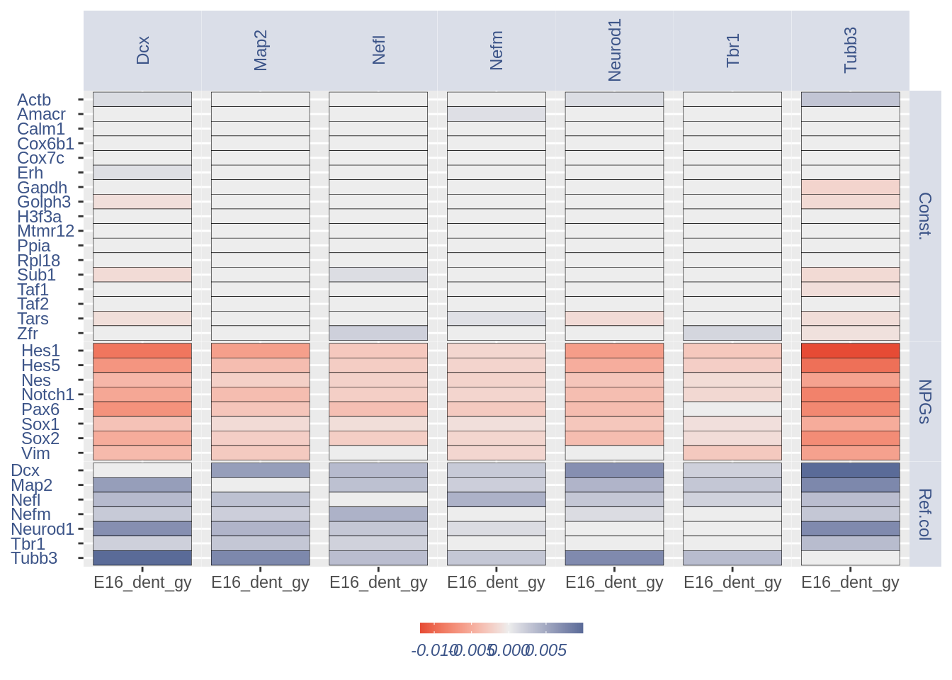
print(sessionInfo())
#> R version 4.0.4 (2021-02-15)
#> Platform: x86_64-pc-linux-gnu (64-bit)
#> Running under: Ubuntu 18.04.5 LTS
#>
#> Matrix products: default
#> BLAS:   /usr/lib/x86_64-linux-gnu/openblas/libblas.so.3
#> LAPACK: /usr/lib/x86_64-linux-gnu/libopenblasp-r0.2.20.so
#>
#> locale:
#>  [1] LC_CTYPE=en_US.UTF-8       LC_NUMERIC=C
#>  [3] LC_TIME=en_US.UTF-8        LC_COLLATE=en_US.UTF-8
#>  [5] LC_MONETARY=en_US.UTF-8    LC_MESSAGES=en_US.UTF-8
#>  [7] LC_PAPER=en_US.UTF-8       LC_NAME=C
#>  [9] LC_ADDRESS=C               LC_TELEPHONE=C
#> [11] LC_MEASUREMENT=en_US.UTF-8 LC_IDENTIFICATION=C
#>
#> attached base packages:
#> [1] stats     graphics  grDevices utils     datasets  methods   base
#>
#> other attached packages:
#> [1] latex2exp_0.5.0   ggrepel_0.9.1     ggplot2_3.3.3     Matrix_1.3-2
#> [5] data.table_1.14.0 COTAN_0.1.0
#>
#> loaded via a namespace (and not attached):
#>  [1] Rcpp_1.0.6           lattice_0.20-41      circlize_0.4.12
#>  [4] tidyr_1.1.2          png_0.1-7            assertthat_0.2.1
#>  [7] digest_0.6.27        utf8_1.2.1           R6_2.5.0
#> [10] stats4_4.0.4         evaluate_0.14        highr_0.8
#> [13] pillar_1.5.1         basilisk_1.2.1       GlobalOptions_0.1.2
#> [16] rlang_0.4.10         jquerylib_0.1.3      S4Vectors_0.28.1
#> [19] GetoptLong_1.0.5     reticulate_1.18      rmarkdown_2.7
#> [22] labeling_0.4.2       stringr_1.4.0        munsell_0.5.0
#> [25] compiler_4.0.4       xfun_0.22            pkgconfig_2.0.3
#> [28] BiocGenerics_0.36.0  shape_1.4.5          htmltools_0.5.1.1
#> [31] tidyselect_1.1.0     tibble_3.1.0         IRanges_2.24.1
#> [34] matrixStats_0.58.0   fansi_0.4.2          withr_2.4.1
#> [37] crayon_1.4.0         dplyr_1.0.4          rappdirs_0.3.3
#> [40] basilisk.utils_1.2.2 grid_4.0.4           gtable_0.3.0
#> [43] jsonlite_1.7.2       lifecycle_1.0.0      DBI_1.1.1
#> [46] magrittr_2.0.1       formatR_1.8          scales_1.1.1
#> [49] stringi_1.5.3        farver_2.1.0         bslib_0.2.4
#> [52] ellipsis_0.3.1       filelock_1.0.2       generics_0.1.0
#> [55] vctrs_0.3.6          cowplot_1.1.1        rjson_0.2.20
#> [58] RColorBrewer_1.1-2   tools_4.0.4          Cairo_1.5-12.2
#> [61] glue_1.4.2           purrr_0.3.4          parallel_4.0.4
#> [64] yaml_2.2.1           clue_0.3-58          colorspace_2.0-0
#> [67] cluster_2.1.1        ComplexHeatmap_2.6.2 knitr_1.31
#> [70] sass_0.3.1