P0 cortex
library(COTAN)
library(data.table)
library(Matrix)
library(ggrepel)
#> Loading required package: ggplot2
# library(latex2exp)
mycolours <- c(A = "#8491B4B2", B = "#E64B35FF")
my_theme = theme(axis.text.x = element_text(size = 14,
angle = 0, hjust = 0.5, vjust = 0.5,
face = "plain", colour = "#3C5488FF"),
axis.text.y = element_text(size = 14,
angle = 0, hjust = 0, vjust = 0.5,
face = "plain", colour = "#3C5488FF"),
axis.title.x = element_text(size = 14,
angle = 0, hjust = 0.5, vjust = 0,
face = "plain", colour = "#3C5488FF"),
axis.title.y = element_text(size = 14,
angle = 90, hjust = 0.5, vjust = 0.5,
face = "plain", colour = "#3C5488FF"))data = as.data.frame(fread(paste(data_dir,
"GSE123335_P0_combined_matrix.txt.gz",
sep = "/")))
data = as.data.frame(data)
rownames(data) = data$Gene
data = data[, 2:ncol(data)]
data[1:10, 1:10]
#> p0-WT2_AAAACATGAACC p0-WT2_AAAAGACACCAC p0-WT2_AAAAGGCTCGTG
#> 0610005C13Rik 0 0 0
#> 0610007N19Rik 0 0 0
#> 0610007P14Rik 0 0 0
#> 0610009B22Rik 0 0 0
#> 0610009D07Rik 0 0 0
#> 0610009E02Rik 0 0 0
#> 0610009L18Rik 0 0 0
#> 0610009O20Rik 0 0 0
#> 0610010F05Rik 0 3 1
#> 0610010K14Rik 0 0 0
#> p0-WT2_AAAATACGCAAG p0-WT2_AAACACCGGATA p0-WT2_AAACACCGGGCA
#> 0610005C13Rik 0 0 0
#> 0610007N19Rik 0 0 0
#> 0610007P14Rik 0 3 0
#> 0610009B22Rik 0 1 0
#> 0610009D07Rik 1 0 1
#> 0610009E02Rik 0 0 0
#> 0610009L18Rik 0 0 0
#> 0610009O20Rik 0 0 0
#> 0610010F05Rik 0 0 0
#> 0610010K14Rik 0 0 0
#> p0-WT2_AAACAGGTCCGT p0-WT2_AAACCATCACTA p0-WT2_AAACCTACTCTT
#> 0610005C13Rik 0 0 0
#> 0610007N19Rik 0 0 0
#> 0610007P14Rik 1 0 0
#> 0610009B22Rik 1 1 1
#> 0610009D07Rik 0 0 3
#> 0610009E02Rik 0 2 0
#> 0610009L18Rik 0 0 0
#> 0610009O20Rik 0 1 0
#> 0610010F05Rik 0 0 0
#> 0610010K14Rik 0 0 0
#> p0-WT2_AAACCTCATTTC
#> 0610005C13Rik 0
#> 0610007N19Rik 0
#> 0610007P14Rik 0
#> 0610009B22Rik 0
#> 0610009D07Rik 1
#> 0610009E02Rik 0
#> 0610009L18Rik 0
#> 0610009O20Rik 0
#> 0610010F05Rik 0
#> 0610010K14Rik 0Define a directory where the ouput will be stored.
0.1 Analytical pipeline
Initialize the COTAN object with the row count table and the metadata for the experiment.
obj = new("scCOTAN", raw = data)
obj = initRaw(obj, GEO = "GSE123335", sc.method = "10X",
    cond = "mouse cortex P0")
#> [1] "Initializing S4 object"
Now we can start the cleaning. Analysis requires and starts from a matrix of raw UMI counts after removing possible cell doublets or multiplets and low quality or dying cells (with too high mtRNA percentage, easily done with Seurat or other tools).
If we do not want to consider the mitochondrial genes we can remove them before starting the analysis.
genes_to_rem = rownames(obj@raw[grep("^mt",
    rownames(obj@raw)), ])  #genes to remove : mithocondrial
obj@raw = obj@raw[!rownames(obj@raw) %in%
    genes_to_rem, ]
cells_to_rem = colnames(obj@raw[which(colSums(obj@raw) ==
    0)])
obj@raw = obj@raw[, !colnames(obj@raw) %in%
    cells_to_rem]
We want also to define a prefix to identify the sample.
0.2 Data cleaning
First we create the directory to store all information regardin the data cleaning.
if (!file.exists(out_dir)) {
    dir.create(file.path(out_dir))
}

if (!file.exists(paste(out_dir, "cleaning",
    sep = ""))) {
    dir.create(file.path(out_dir, "cleaning"))
}
ttm = clean(obj)
#> [1] "Start estimation mu with linear method"
#> [1] 14438 7688
#> rowname p0-WT2_ACGAGCGATAGA p0-WT2_CAATCAGTTCAT p0-WT2_CAGTACCACATA
#> 8624 Npy 269.054089 260.832176 420.693732
#> 12065 Sst 102.371800 78.642867 102.935700
#> 13263 Tuba1a 18.374426 9.175001 19.393683
#> 7440 Malat1 36.748851 0.000000 1.491822
#> 8551 Nnat 26.249179 18.350002 17.901861
#> 7679 Meg3 26.249179 3.932143 0.000000
#> 847 Actb 22.311802 13.107145 10.442752
#> 2115 Calm1 6.562295 7.864287 13.426396
#> 9101 Pcp4 0.000000 6.553572 5.967287
#> 6352 Hsp90ab1 6.562295 19.660717 5.967287
#> 10893 Rtn1 11.812131 22.282146 4.475465
#> 4921 Gap43 5.249836 7.864287 11.934574
#> 5762 Gnas 1.312459 11.796430 13.426396
#> 7530 Mapt 5.249836 5.242858 13.426396
#> 12890 Tmsb4x 7.874754 1.310714 4.475465
#> p0-WT2_TCAGCCAGGCAT p0-WT3_ACCAATCGACAG p0-WT3_ATCTCTTGCTGG
#> 8624 165.023143 198.814905 158.297051
#> 12065 87.365193 46.841208 47.659327
#> 13263 53.389840 11.450073 25.531782
#> 7440 0.000000 31.227472 6.808475
#> 8551 26.694920 14.572820 11.914832
#> 7679 0.000000 12.490989 0.000000
#> 847 24.268109 15.613736 8.510594
#> 2115 12.134055 6.245494 18.723307
#> 9101 19.414487 16.654652 0.000000
#> 6352 4.853622 7.286410 13.616951
#> 10893 7.280433 5.204579 6.808475
#> 4921 4.853622 13.531905 17.021188
#> 5762 4.853622 10.409157 6.808475
#> 7530 4.853622 3.122747 11.914832
#> 12890 9.707244 1.040916 15.319069
#> p0-WT3_GGATTGACAGGA p0-WT3_GTGAGATTCGAA p0-WT3_TACCGATCAAAG
#> 8624 227.695969 89.091134 194.188936
#> 12065 72.368486 189.604208 41.316795
#> 13263 12.355595 31.981433 26.167303
#> 7440 1.765085 41.118985 13.772265
#> 8551 24.711190 15.990716 15.149491
#> 7679 0.000000 38.834597 20.658397
#> 847 10.590510 9.137552 22.035624
#> 2115 3.530170 18.275104 15.149491
#> 9101 17.650850 4.568776 19.281171
#> 6352 7.060340 4.568776 12.395038
#> 10893 5.295255 4.568776 8.263359
#> 4921 8.825425 0.000000 5.508906
#> 5762 5.295255 15.990716 4.131679
#> 7530 7.060340 2.284388 5.508906
#> 12890 8.825425 2.284388 0.000000
#> p0-WT3_TGAGGAATGAGA p0-WT4_CCGCAAAGCACT p0-WT4_TCCTTTAACCTT
#> 8624 240.738358 175.421286 162.138055
#> 12065 78.379930 57.861471 58.467965
#> 13263 13.436560 25.716209 16.213806
#> 7440 23.513979 16.531849 37.340885
#> 8551 8.957706 33.063698 20.144425
#> 7679 15.675986 20.205593 21.127080
#> 847 10.077420 11.021233 9.335221
#> 2115 12.316846 3.673744 3.930620
#> 9101 2.239427 6.429052 4.913274
#> 6352 10.077420 5.510616 1.965310
#> 10893 6.718280 8.265924 10.809204
#> 4921 7.837993 5.510616 8.843894
#> 5762 2.239427 1.836872 5.404602
#> 7530 4.478853 8.265924 3.439292
#> 12890 5.598566 13.776541 9.335221
#> p0-WT4_TCGTGGTCGTCA
#> 8624 260.0206889
#> 12065 65.6617901
#> 13263 14.8833391
#> 7440 59.5333564
#> 8551 14.0078486
#> 7679 38.5215835
#> 847 2.6264716
#> 2115 6.1284337
#> 9101 12.2568675
#> 6352 13.1323580
#> 10893 10.5058864
#> 4921 6.1284337
#> 5762 3.5019621
#> 7530 6.1284337
#> 12890 0.8754905
obj = ttm$object
ttm$pca.cell.2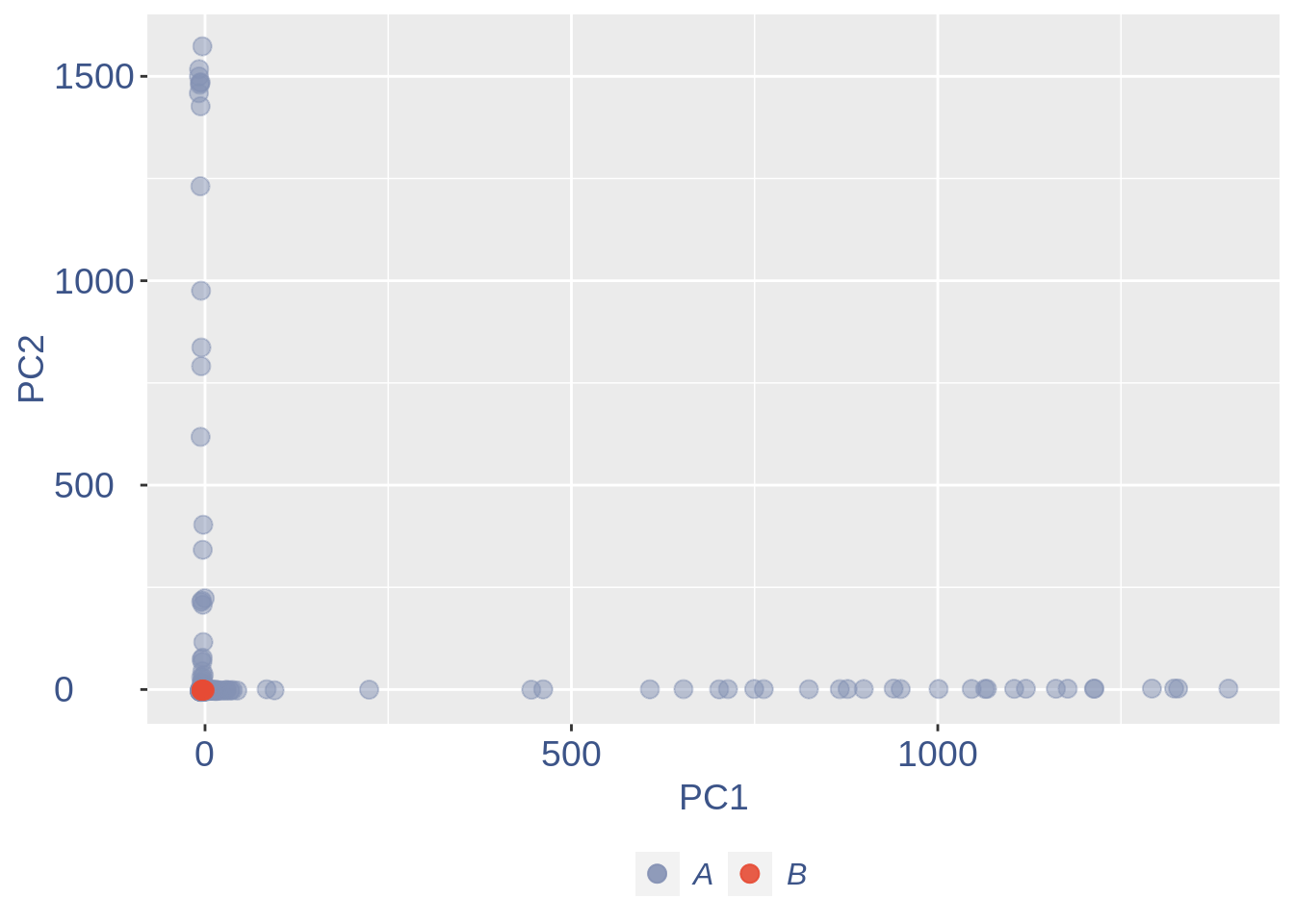
Run this when B cells need to be removed.
pdf(paste(out_dir, "cleaning/", t, "_", n_it,
    "_plots_before_cells_exlusion.pdf", sep = ""))
ttm$pca.cell.2
ggplot(ttm$D, aes(x = n, y = means)) + geom_point() +
    geom_text_repel(data = subset(ttm$D,
        n > (max(ttm$D$n) - 15)), aes(n,
        means, label = rownames(ttm$D[ttm$D$n >
            (max(ttm$D$n) - 15), ])), nudge_y = 0.05,
        nudge_x = 0.05, direction = "x",
        angle = 90, vjust = 0, segment.size = 0.2) +
    ggtitle("B cell group genes mean expression") +
    my_theme + theme(plot.title = element_text(color = "#3C5488FF",
    size = 20, face = "italic", vjust = -5,
    hjust = 0.02))
dev.off()
#> png
#>   2

if (length(ttm$cl1) < length(ttm$cl2)) {
    to_rem = ttm$cl1
} else {
    to_rem = ttm$cl2
}
n_it = n_it + 1
obj@raw = obj@raw[, !colnames(obj@raw) %in%
    to_rem]
gc()
#>             used   (Mb) gc trigger   (Mb)   max used   (Mb)
#> Ncells   3759604  200.8    6027441  322.0    6027441  322.0
#> Vcells 740559876 5650.1 1217801675 9291.1 1014763509 7742.1

ttm = clean(obj)
#> [1] "Start estimation mu with linear method"
#> [1] 14433  7675
#>       rowname p0-WT2_ACCGCAGAGGGC p0-WT2_CCCTAACCCCAT p0-WT2_CGGTCGTACACT
#> 6103   Hbb-bs          1510.26571         1360.067486          598.326652
#> 6104   Hbb-bt           304.31935          421.429362          127.944064
#> 6101   Hba-a1           335.07503          354.947190          110.383114
#> 6102   Hba-a2           168.34687          233.251010           66.480739
#> 5912     Gpx1            50.18032            3.380449            3.763061
#> 7439   Malat1             3.23744            1.126816           46.411082
#> 1071    Alas2            17.80592           11.268165            2.508707
#> 4804     Fth1             8.09360            5.634082            5.017414
#> 8927   Pabpc1            19.42464            0.000000            0.000000
#> 13259  Tuba1a             1.61872            0.000000           20.069657
#> 847      Actb             3.23744            0.000000           17.560950
#> 1930     Bpgm             4.85616            3.380449            2.508707
#> 7836    Mkrn1             8.09360            1.126816            0.000000
#> 11747    Snca             3.23744            5.634082            1.254354
#> 12887  Tmsb4x             0.00000            1.126816            7.526121
#>       p0-WT2_CTACTTGCCCGT p0-WT2_TCACGACGTTTN p0-WT2_TTACGACTCGAN
#> 6103          919.7849387         1393.879227         1376.342017
#> 6104          215.7520227          278.300119          406.908486
#> 6101          223.3222691          271.164218          352.730869
#> 6102          139.1032778          259.271051          263.971794
#> 5912           16.0867736            9.514534           20.748875
#> 7439           77.5950257            0.000000            0.000000
#> 1071            2.8388424           16.650434           18.443444
#> 4804            4.7314040            2.378633            2.305431
#> 8927            3.7851232            4.757267            1.152715
#> 13259           7.5702464            7.135900            5.763576
#> 847             3.7851232            2.378633            3.458146
#> 1930            2.8388424            4.757267            3.458146
#> 7836            0.9462808            0.000000            2.305431
#> 11747           1.8925616            2.378633            4.610861
#> 12887           0.9462808            4.757267            3.458146
#>       p0-WT3_AGAGGTGCTAGT p0-WT3_CTCCTAACGGAC p0-WT4_CAATACCGTAAC
#> 6103          1347.979875        1093.5829767          726.090046
#> 6104           467.299690         391.0924276          224.548702
#> 6101           464.031860         334.2733390          200.173349
#> 6102           266.328145         254.5790330          108.581116
#> 5912             6.535660          25.0889482            2.954588
#> 7439             0.000000          25.0889482            1.477294
#> 1071             8.169575           9.5928331            8.125118
#> 4804             8.169575          16.9719355            5.909176
#> 8927             0.000000          19.9235765            1.477294
#> 13259            1.633915           0.7379102           14.034294
#> 847              1.633915           4.4274614           14.772941
#> 1930             1.633915          10.3307434            0.000000
#> 7836             3.267830          12.5444741            2.954588
#> 11747            4.901745           0.0000000            2.954588
#> 12887            1.633915           2.9516410            8.125118
#>       p0-WT4_CTGAGTAACTTT p0-WT4_GCGGGCCTCTCG p0-WT4_GGACCACCATGA
#> 6103         1313.4473803          784.999535         1256.898569
#> 6104          543.8199039          192.967158          545.398085
#> 6101          332.1253046          187.258071          347.616362
#> 6102          286.0229252          127.312652          250.865995
#> 5912            5.6451893            3.425453           29.110730
#> 7439            0.9408649           11.418175            0.000000
#> 1071           12.2312435            5.138179           17.123959
#> 4804            7.5269191           16.556354            7.705781
#> 8927            5.6451893            5.709088            9.418177
#> 13259           1.8817298            2.854544            4.280990
#> 847             0.9408649            6.279996            3.424792
#> 1930            0.9408649            3.425453           11.130573
#> 7836            1.8817298            3.425453           10.274375
#> 11747           1.8817298            1.141818           11.986771
#> 12887           3.7634595           10.276358            3.424792
#>       p0-WT4_TTGAAACTTTTC
#> 6103          1332.664320
#> 6104           502.117599
#> 6101           353.692900
#> 6102           254.743101
#> 5912             5.263287
#> 7439             4.210630
#> 1071             8.421260
#> 4804            10.526574
#> 8927             4.210630
#> 13259            2.105315
#> 847              5.263287
#> 1930             2.105315
#> 7836             4.210630
#> 11747            6.315945
#> 12887            0.000000
obj = ttm$object

ttm$pca.cell.2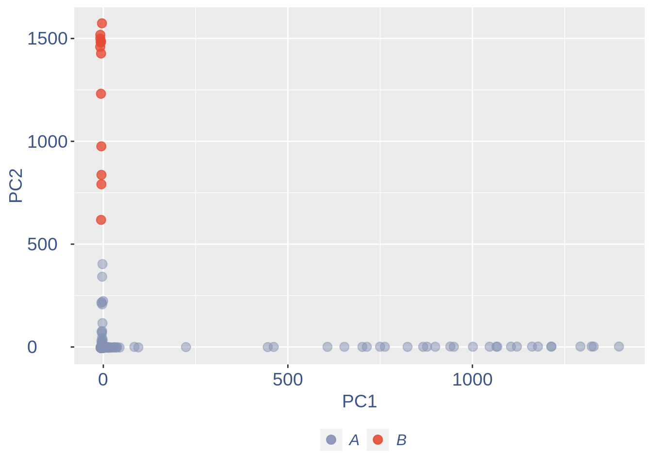
#> png
#>   2
#>             used   (Mb) gc trigger    (Mb)   max used    (Mb)
#> Ncells   3759877  200.8    6027441   322.0    6027441   322.0
#> Vcells 759014948 5790.9 1753810412 13380.6 1753805348 13380.5
#> [1] "Start estimation mu with linear method"
#> [1] 14432  7662
#>             rowname p0-WT2_AAGAAAGACTCN p0-WT2_AAGAATAGACTC p0-WT2_ACGCTTAGATCT
#> 13254           Ttr         1217.302279         1123.775923          752.020748
#> 7439         Malat1            0.000000            2.493586           32.621023
#> 62    1500015O10Rik           11.226767           14.130319           18.337262
#> 1294           Apoe            0.000000            6.649562           21.811690
#> 6477         Igfbp2           16.038238            9.974343            9.651190
#> 1971            Bsg           14.434414            9.974343           11.002357
#> 1413        Arl6ip1           17.642062           14.130319           13.511666
#> 847            Actb           12.830591           20.779880            9.844214
#> 4804           Fth1           20.849710           18.286295            7.913976
#> 3142           Cst3            9.622943            7.480757            8.493047
#> 2817            Clu            1.603824            3.324781            5.983738
#> 3000         Cox4i1            4.811471            7.480757            4.439548
#> 11905         Sparc            1.603824            4.155976            9.651190
#> 5761           Gnas           11.226767            3.324781            3.281405
#> 4138          Enpp2            0.000000            2.493586           11.967476
#>       p0-WT2_ACGTTCCCCGTC p0-WT2_ATCCACGGAGCN p0-WT2_ATTAGGGTCAAG
#> 13254          764.941504          952.234482          901.949597
#> 7439            23.131518           29.243285           23.358501
#> 62              17.081736           14.621643            8.097614
#> 1294            18.861084           31.070991           22.424161
#> 6477            16.725867           18.277053            6.228934
#> 1971            16.014128           14.621643           11.523527
#> 1413             9.252607           10.966232           15.260888
#> 847              5.338043            7.310821           11.212081
#> 4804             9.786411            3.655411            5.917487
#> 3142             4.982173           12.793937            6.851827
#> 2817            10.142281            0.000000            5.294594
#> 3000             5.160108           16.449348            5.606040
#> 11905            7.651194            1.827705           11.212081
#> 5761             6.049782            1.827705            2.180127
#> 4138             6.405651            1.827705            5.917487
#>       p0-WT2_GTCATTCCTCTC p0-WT2_GTCTTATTAGTA p0-WT2_TTAATAGAATCT
#> 13254          869.287587         1164.869643          704.390419
#> 7439            41.957614           15.891810           36.911288
#> 62              10.199641            7.945905           30.759407
#> 1294             8.345161            6.356724            9.227822
#> 6477            13.676791           14.302629            6.151881
#> 1971            14.835841           11.124267            1.537970
#> 1413             7.417921            9.535086           12.303763
#> 847              6.490681            7.945905            6.151881
#> 4804             6.722491           11.124267            3.075941
#> 3142             7.417921            7.945905            0.000000
#> 2817            12.054121            9.535086            9.227822
#> 3000             4.172580            6.356724           12.303763
#> 11905           13.444981            3.178362            1.537970
#> 5761             3.940770            4.767543            4.613911
#> 4138             6.258871            6.356724           16.917674
#>       p0-WT3_AAATCTGCTGGA p0-WT3_AAGTAATAGCAC p0-WT3_AATAGCCGGATG
#> 13254         1070.650373         1107.917463         1217.527817
#> 7439            13.917776           21.452791            0.000000
#> 62              14.936150           10.488031           10.274496
#> 1294             7.468075            8.581116            2.568624
#> 6477             7.128617           12.394946           10.274496
#> 1971             9.165365           11.441488            2.568624
#> 1413            13.238860           11.441488            2.568624
#> 847             11.202112            8.104388           12.843120
#> 4804             8.825907            3.813829            2.568624
#> 3142             8.146991            9.534574            7.705872
#> 2817             7.807533            4.290558            2.568624
#> 3000             6.789159            7.150930            7.705872
#> 11905            3.734037            6.197473            2.568624
#> 5761             6.449701            5.720744            5.137248
#> 4138             4.412953            7.627659            2.568624
#>       p0-WT3_AGTAAATGCCGG p0-WT3_CTTTTCAATATG p0-WT3_GACGTTCCCGCA
#> 13254         1067.929605         1331.918004          609.055540
#> 7439            25.175972            1.716389           20.954534
#> 62              14.637193            1.716389           30.916525
#> 1294            22.248533           17.163892           21.641567
#> 6477             5.854877            8.581946           15.458262
#> 1971             8.196828           15.447503           11.679576
#> 1413             7.025853            6.865557           16.488813
#> 847              4.098414           10.298335            5.839788
#> 4804             8.196828            5.149168            8.931441
#> 3142             2.341951            6.865557            8.587924
#> 2817             7.611340            6.865557           17.519364
#> 3000             2.341951            5.149168            4.122203
#> 11905            8.782316            3.432778           18.206398
#> 5761             5.269389            5.149168            8.244407
#> 4138             6.440365            1.716389            5.496271
#>       p0-WT3_GCGTTGTAGCAG p0-WT3_TCTGGCCGCACT p0-WT3_TGGGCGTTCCCG
#> 13254         1326.094995         1049.745426          943.212474
#> 7439             0.000000           34.982260           23.031932
#> 62              15.343248           11.938390            3.290276
#> 1294            13.151355            6.663288           18.644898
#> 6477            26.302711           11.660753           12.064346
#> 1971            10.959463           12.216027            9.870828
#> 1413             8.767570            7.773835            9.870828
#> 847              4.383785            6.940925           10.967587
#> 4804             4.383785            6.663288            6.580552
#> 3142             0.000000            8.606746           10.967587
#> 2817             4.383785            5.275103            6.580552
#> 3000             4.383785            7.496198            4.387035
#> 11905            2.191893            3.054007            1.096759
#> 5761            13.151355            5.830377            5.483793
#> 4138             4.383785            8.051472           13.161104
#>       p0-WT3_TTAGGCTTCCCG p0-WT4_CCCATACTGTAG p0-WT4_GCGACGGATATT
#> 13254         1401.048190         1296.302791          879.780671
#> 7439            33.450186            1.893795           25.312508
#> 62              10.292365           10.415873           17.559127
#> 1294             5.146183            3.787590           17.787168
#> 6477            14.152002           11.362771           11.630071
#> 1971             9.005819            7.575181           12.314193
#> 1413             9.005819            9.468976           12.770274
#> 847             11.578911            6.628283            4.104731
#> 4804             3.859637            4.734488            7.297299
#> 3142             5.146183            5.681385            4.788853
#> 2817             6.432728            5.681385           10.033787
#> 3000             0.000000            4.734488            8.209462
#> 11905            6.432728            6.628283            6.841218
#> 5761             3.859637            3.787590            4.788853
#> 4138             1.286546            2.840693            3.876690
#>       p0-WT4_TCCAAAGTTGAG p0-WT4_TCCGGAGGGTCC p0-WT4_TCGGAACGGTCC
#> 13254         1004.460920         1180.578131          827.202477
#> 7439            22.938410           20.872100           46.918349
#> 62              14.487417           13.045062           10.929843
#> 1294            15.694702           28.699137           12.262750
#> 6477            10.865563           16.088910           11.463006
#> 1971            12.072848           16.523745            9.330353
#> 1413             7.243709            7.392202            4.265304
#> 847              4.829139            2.609012            5.864794
#> 4804             3.621854            6.522531            6.931120
#> 3142            13.280132            8.696708            5.864794
#> 2817             4.829139            8.696708           11.996169
#> 3000             9.658278            5.652860            3.465560
#> 11905            4.829139           10.001214            8.264027
#> 5761             8.450993            5.218025            5.331631
#> 4138             4.829139            6.087696            2.665815
#>       p0-WT4_TGTATAGGAAAG p0-WT4_TTGTTTTGCACG
#> 13254          655.456794          716.143243
#> 7439            19.988266           17.691844
#> 62              18.009230           12.610144
#> 1294             3.760169            8.281288
#> 6477            13.259543           14.304044
#> 1971             9.499374           13.739410
#> 1413            16.623904           15.997944
#> 847              9.301470            3.387800
#> 4804             8.114048            7.716655
#> 3142             4.749687            7.904866
#> 2817             6.926627            6.210966
#> 3000             6.728723            7.904866
#> 11905            5.145494            5.269911
#> 5761             5.739205            6.210966
#> 4138             8.311952            2.823167
#> png
#>   2
#>             used   (Mb) gc trigger    (Mb)   max used    (Mb)
#> Ncells   3760142  200.9    6027441   322.0    6027441   322.0
#> Vcells 758184164 5784.5 2104652494 16057.3 2104648276 16057.2
#> [1] "Start estimation mu with linear method"
#> [1] 14387  7636
#>       rowname p0-WT2_AACATATAGGTC p0-WT2_CTGCTACCACCA p0-WT2_TTGTTTAGAGAT
#> 7649     Meg3          168.437377           128.87216          143.216174
#> 7410   Malat1          156.740337            96.06834          107.659055
#> 11714  Snhg11            4.678816            42.17634           81.978913
#> 5913    Gria2           11.697040            11.71565           13.827769
#> 8520     Nnat            0.000000             2.34313            9.876978
#> 13216  Tuba1a            4.678816            11.71565            9.876978
#> 10856    Rtn1            4.678816            14.05878            8.889280
#> 8593      Npy            0.000000            18.74504           26.667839
#> 11815     Son            7.018224             2.34313            6.913884
#> 9513      Pnn            7.018224             0.00000            2.963093
#> 11988   Srrm2            7.018224             0.00000            3.950791
#> 1328   Arglu1           14.036448             0.00000            4.938489
#> 5912    Gria1           11.697040             4.68626            7.901582
#> 4711   Fnbp1l            2.339408             0.00000            4.938489
#> 6891    Kif5c            4.678816             4.68626            1.975396
#>       p0-WT3_GCACGTACTAAT p0-WT4_CGTAAACCCAGC
#> 7649           162.409305          282.814854
#> 7410            39.504966          210.091034
#> 11714           13.168322           56.562971
#> 5913            13.168322            8.080424
#> 8520            28.531364           12.120637
#> 13216           10.973602           12.120637
#> 10856            6.584161           12.120637
#> 8593             0.000000            0.000000
#> 11815            4.389441           16.160849
#> 9513            17.557763            8.080424
#> 11988            8.778881           12.120637
#> 1328             2.194720            8.080424
#> 5912             4.389441            0.000000
#> 4711             8.778881           12.120637
#> 6891             4.389441           12.120637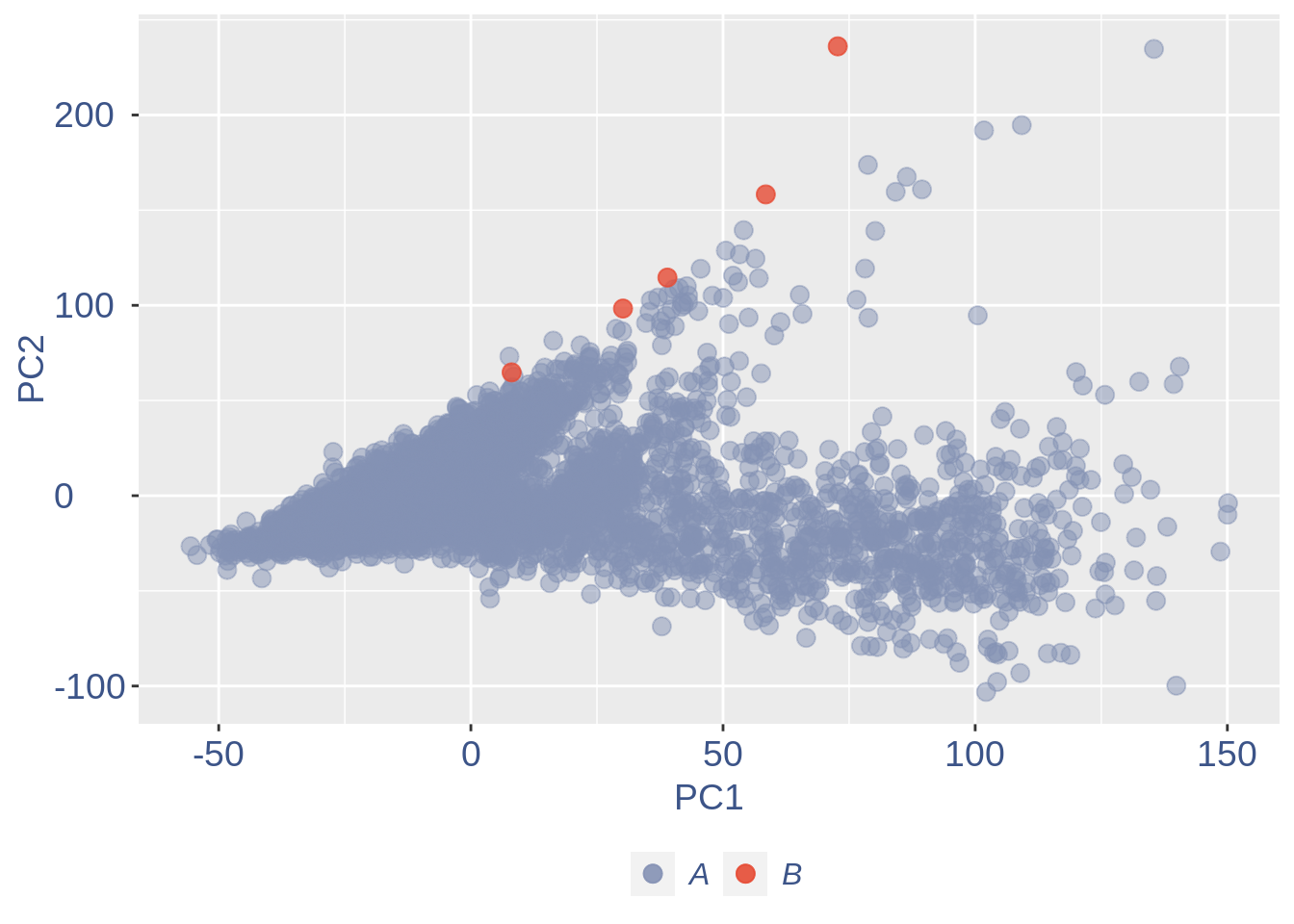
Run this only in the last iteration, instead the previous code, when B cells group has not to be removed.
pdf(paste(out_dir, "cleaning/", t, "_", n_it,
    "_plots_before_cells_exlusion.pdf", sep = ""))
ttm$pca.cell.2
ggplot(ttm$D, aes(x = n, y = means)) + geom_point() +
    geom_text_repel(data = subset(ttm$D,
        n > (max(ttm$D$n) - 15)), aes(n,
        means, label = rownames(ttm$D[ttm$D$n >
            (max(ttm$D$n) - 15), ])), nudge_y = 0.05,
        nudge_x = 0.05, direction = "x",
        angle = 90, vjust = 0, segment.size = 0.2) +
    ggtitle(label = "B cell group genes mean expression",
        subtitle = " - B group NOT removed -") +
    my_theme + theme(plot.title = element_text(color = "#3C5488FF",
    size = 20, face = "italic", vjust = -10,
    hjust = 0.02), plot.subtitle = element_text(color = "darkred",
    vjust = -15, hjust = 0.01))

dev.off()
#> png
#>   2
To color the pca based on nu_j (so the cells’ efficiency).
nu_est = round(obj@nu, digits = 7)

plot.nu <- ggplot(ttm$pca_cells, aes(x = PC1,
    y = PC2, colour = log(nu_est)))

plot.nu = plot.nu + geom_point(size = 1,
    alpha = 0.8) + scale_color_gradient2(low = "#E64B35B2",
    mid = "#4DBBD5B2", high = "#3C5488B2",
    midpoint = log(mean(nu_est)), name = "ln (nu)") +
    ggtitle("Cells PCA coloured by cells efficiency") +
    my_theme + theme(plot.title = element_text(color = "#3C5488FF",
    size = 20), legend.title = element_text(color = "#3C5488FF",
    size = 14, face = "italic"), legend.text = element_text(color = "#3C5488FF",
    size = 11), legend.key.width = unit(2,
    "mm"), legend.position = "right")

pdf(paste(out_dir, "cleaning/", t, "_plots_PCA_efficiency_colored.pdf",
    sep = ""))
plot.nu
dev.off()
#> png
#>   2

plot.nu
The next part is used to remove the cells with efficiency too low.
nu_df = data.frame(nu = sort(obj@nu), n = c(1:length(obj@nu)))

ggplot(nu_df, aes(x = n, y = nu)) + geom_point(colour = "#8491B4B2",
    size = 1) + my_theme  #+ ylim(0,1) + xlim(0,70)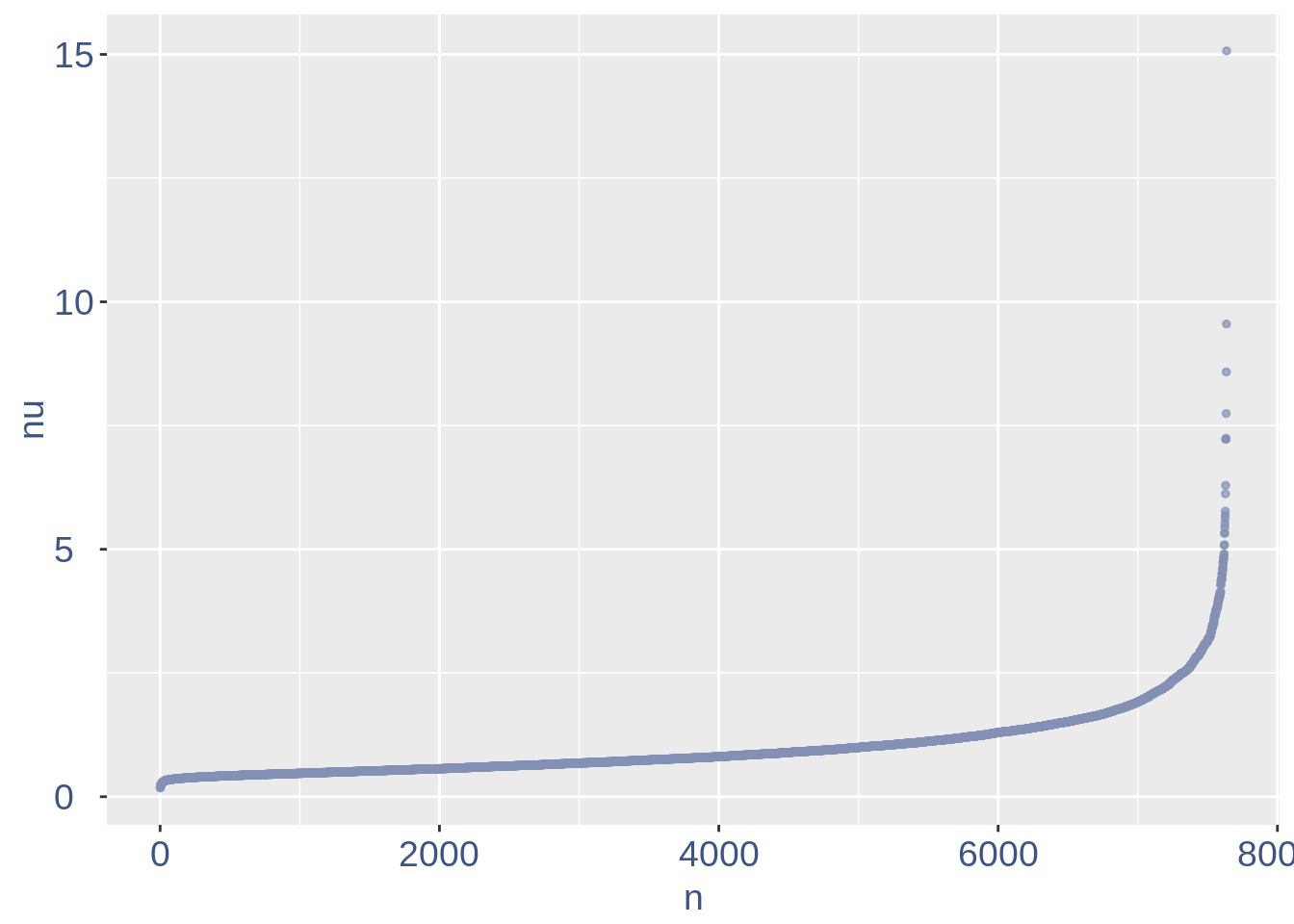
We can zoom on the smallest values and, if we detect a clear elbow, we can decide to remove the cells.
yset = 0.35  #threshold to remove low UDE cells
plot.ude <- ggplot(nu_df, aes(x = n, y = nu)) +
    geom_point(colour = "#8491B4B2", size = 1) +
    my_theme + ylim(0, 0.7) + xlim(0, 2000) +
    geom_hline(yintercept = yset, linetype = "dashed",
        color = "darkred") + annotate(geom = "text",
    x = 500, y = 0.5, label = paste("to remove cells with nu < ",
        yset, sep = " "), color = "darkred",
    size = 4.5)


pdf(paste(out_dir, "cleaning/", t, "_plots_efficiency.pdf",
    sep = ""))
plot.ude
dev.off()
#> png
#>   2

plot.ude
We also save the defined threshold in the metadata and re-run the estimation.
obj@meta[(nrow(obj@meta) + 1), 1:2] = c("Threshold low UDE cells:",
    yset)

to_rem = rownames(nu_df[which(nu_df$nu <
    yset), ])

obj@raw = obj@raw[, !colnames(obj@raw) %in%
    to_rem]
Repeat the estimation after the cells are removed
ttm = clean(obj)
#> [1] "Start estimation mu with linear method"
#> [1] 14382  7554
#>       rowname p0-WT2_AAAGTGCTAGCC p0-WT2_GAAGTTAGGGAN p0-WT2_GATCTAGCGTGG
#> 1287     Apoe           277.40779          270.637698          273.898393
#> 12839  Tmsb4x            42.12655           42.389037           62.922604
#> 3169     Ctsd            95.45696           44.019385            7.402659
#> 3167     Ctsb            52.43411           45.649732           11.103989
#> 841      Actb            25.54482           39.128342           43.182179
#> 3127     Cst3            30.02637           37.497994           12.337765
#> 2009     C1qb            17.02988           35.867647           25.909307
#> 2011     C1qc            22.85589           30.976604           25.909307
#> 4784     Fth1            28.23375            9.782085            9.870212
#> 1667      B2m            18.37434           32.606952           18.506648
#> 7102     Lgmn            18.37434           37.497994            8.636436
#> 13273  Tyrobp            18.82250           17.933823            6.168883
#> 7406   Malat1             9.41125            1.630348           11.103989
#> 10672  Rpl13a            12.54833           21.194519           13.571542
#> 11117   Sepp1            12.54833           13.042781            6.168883
#>       p0-WT2_GATCTAGCGTGN p0-WT2_GGATCCGCCCAA p0-WT3_AACAGTGCAGAA
#> 1287           229.480218          285.411229          270.247259
#> 12839           67.598824           97.457493           32.923524
#> 3169             5.336749           29.585310           12.346321
#> 3167             7.115666           27.844998            9.602694
#> 841             23.125913           43.507809           16.461762
#> 3127            12.452415           31.325623           27.436270
#> 2009            37.357245           24.364373           20.577202
#> 2011            17.789164           19.143436           17.833575
#> 4784            17.789164           22.624061           17.833575
#> 1667            16.010248           17.403124           10.974508
#> 7102             3.557833            8.701562           10.974508
#> 13273           10.673499           13.922499           15.089948
#> 7406            10.673499            8.701562           12.346321
#> 10672           10.673499            6.961249           19.205389
#> 11117            5.336749            5.220937            9.602694
#>       p0-WT3_GCCTTCCTCCGA
#> 1287           227.176931
#> 12839           57.665013
#> 3169            72.758540
#> 3167            56.890986
#> 841             16.254567
#> 3127            37.540311
#> 2009            18.189635
#> 2011            26.703932
#> 4784            22.059770
#> 1667            13.545473
#> 7102            13.545473
#> 13273           17.802622
#> 7406            40.249405
#> 10672            9.288324
#> 11117           41.023432
obj = ttm$object
ttm$pca.cell.2
Just to check again, we plot the final efficiency colored PCA
nu_est = round(obj@nu, digits = 7)
plot.nu <- ggplot(ttm$pca_cells, aes(x = PC1,
    y = PC2, colour = log(nu_est)))
plot.nu = plot.nu + geom_point(size = 2,
    alpha = 0.8) + scale_color_gradient2(low = "#E64B35B2",
    mid = "#4DBBD5B2", high = "#3C5488B2",
    midpoint = log(mean(nu_est)), name = "ln(nu)") +
    ggtitle("Cells PCA coloured by cells efficiency: last") +
    my_theme + theme(plot.title = element_text(color = "#3C5488FF",
    size = 20), legend.title = element_text(color = "#3C5488FF",
    size = 14, face = "italic"), legend.text = element_text(color = "#3C5488FF",
    size = 11), legend.key.width = unit(2,
    "mm"), legend.position = "right")

pdf(paste(out_dir, "cleaning/", t, "_plots_PCA_efficiency_colored_FINAL.pdf",
    sep = ""))
plot.nu
dev.off()
#> png
#>   2

plot.nu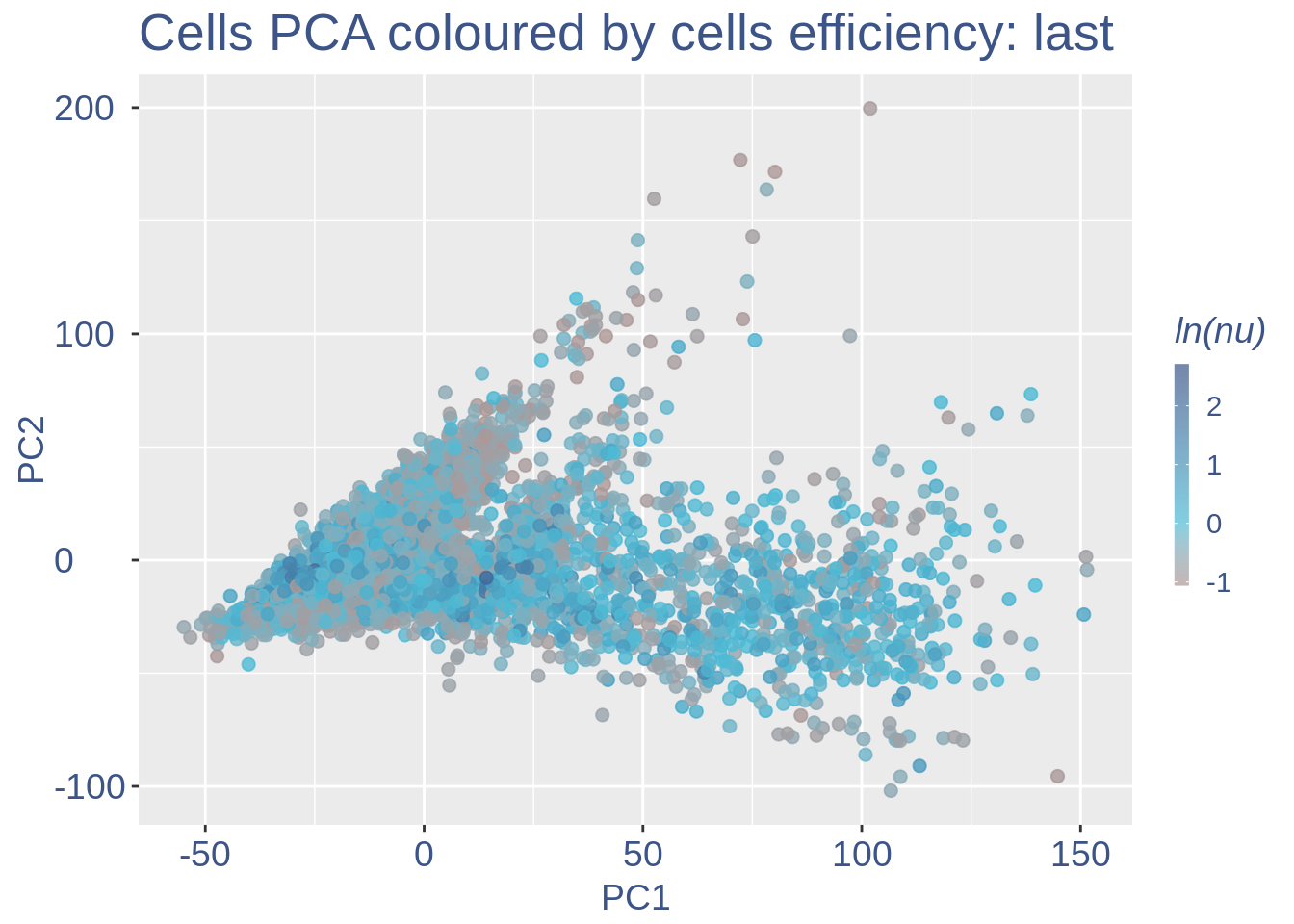
COTAN analysis: in this part all the contingency tables are computed and used to get the statistics (S) To storage efficiency of all the observed tables only the yes_yes is stored. Note that if will be necessary re-computing the yes-yes table, the yes-yes table should be cancelled before running cotan_analysis.
COEX evaluation and storing
0.3 Analysis of the elaborated data
0.3.1 GDI
The next function can directly plot the GDI for the dataset with the 1.5 threshold (in red) and the two higher quantiles (in blue).
plot_GDI(obj, cond = "P0")
#> [1] "GDI plot "
#> [1] "function to generate GDI dataframe"
#> [1] "Using S"
#> [1] "function to generate S "
If a more complex plot is needed, or if we want to analyze mor in detail the GDI data, we can get directly the GDI data frame.
quant.p = get.GDI(obj)
#> [1] "function to generate GDI dataframe"
#> [1] "Using S"
#> [1] "function to generate S "

head(quant.p)
#>               sum.raw.norm      GDI  exp.cells
#> 0610005C13Rik     3.439025 1.261301  0.3177125
#> 0610007N19Rik     5.352070 2.599832  2.0916071
#> 0610007P14Rik     7.718572 2.070818 23.1135822
#> 0610009B22Rik     7.075439 2.047966 13.5954461
#> 0610009D07Rik     8.811660 1.861726 51.6944665
#> 0610009E02Rik     4.905004 2.297613  1.7209425
In the third column of this dataframe is reported the percentage of cells expressing the gene.
NPGs = c("Nes", "Vim", "Sox2", "Sox1", "Notch1",
    "Hes1", "Hes5", "Pax6")  #,'Hes3'
PNGs = c("Map2", "Tubb3", "Neurod1", "Nefm",
    "Nefl", "Dcx", "Tbr1")
hk = c("Calm1", "Cox6b1", "Ppia", "Rpl18",
    "Cox7c", "Erh", "H3f3a", "Taf1", "Taf2",
    "Gapdh", "Actb", "Golph3", "Mtmr12",
    "Zfr", "Sub1", "Tars", "Amacr")

text.size = 12

quant.p$highlight = with(quant.p, ifelse(rownames(quant.p) %in%
    NPGs, "NPGs", ifelse(rownames(quant.p) %in%
    hk, "Constitutive", ifelse(rownames(quant.p) %in%
    PNGs, "PNGs", "normal"))))

textdf <- quant.p[rownames(quant.p) %in%
    c(NPGs, hk, PNGs), ]
mycolours <- c(Constitutive = "#00A087FF",
    NPGs = "#E64B35FF", PNGs = "#F39B7FFF",
    normal = "#8491B4B2")
f1 = ggplot(subset(quant.p, highlight ==
    "normal"), aes(x = sum.raw.norm, y = GDI)) +
    geom_point(alpha = 0.1, color = "#8491B4B2",
        size = 2.5)
GDI_plot = f1 + geom_point(data = subset(quant.p,
    highlight != "normal"), aes(x = sum.raw.norm,
    y = GDI, colour = highlight), size = 2.5,
    alpha = 0.8) + geom_hline(yintercept = quantile(quant.p$GDI)[4],
    linetype = "dashed", color = "darkblue") +
    geom_hline(yintercept = quantile(quant.p$GDI)[3],
        linetype = "dashed", color = "darkblue") +
    geom_hline(yintercept = 1.5, linetype = "dotted",
        color = "red", size = 0.5) + scale_color_manual("Status",
    values = mycolours) + scale_fill_manual("Status",
    values = mycolours) + xlab("log normalized counts") +
    ylab("GDI") + geom_label_repel(data = textdf,
    aes(x = sum.raw.norm, y = GDI, label = rownames(textdf),
        fill = highlight), label.size = NA,
    alpha = 0.5, direction = "both", na.rm = TRUE,
    seed = 1234) + geom_label_repel(data = textdf,
    aes(x = sum.raw.norm, y = GDI, label = rownames(textdf)),
    label.size = NA, segment.color = "black",
    segment.size = 0.5, direction = "both",
    alpha = 0.8, na.rm = TRUE, fill = NA,
    seed = 1234) + theme(axis.text.x = element_text(size = text.size,
    angle = 0, hjust = 0.5, vjust = 0.5,
    face = "plain", colour = "#3C5488FF"),
    axis.text.y = element_text(size = text.size,
        angle = 0, hjust = 0, vjust = 0.5,
        face = "plain", colour = "#3C5488FF"),
    axis.title.x = element_text(size = text.size,
        angle = 0, hjust = 0.5, vjust = 0,
        face = "plain", colour = "#3C5488FF"),
    axis.title.y = element_text(size = text.size,
        angle = 90, hjust = 0.5, vjust = 0.5,
        face = "plain", colour = "#3C5488FF"),
    legend.title = element_blank(), legend.text = element_text(color = "#3C5488FF",
        face = "italic"), legend.position = "bottom")  # titl)
legend <- cowplot::get_legend(GDI_plot)
GDI_plot = GDI_plot + theme(legend.position = "none")
GDI_plot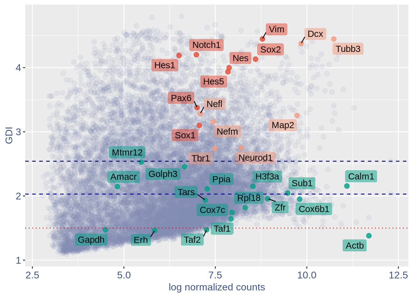
0.3.2 Heatmaps
For the Gene Pair Analysis, we can plot an heatmap with the coex values between two genes sets. To do so we need to define, in a list, the different gene sets (list.genes). Then in the function parameter sets we can decide which sets need to be considered (in the example from 1 to 3). In the condition parameter we should insert an array with each file name prefix to be considered (in the example, the file names is “P0_cortex”).
list.genes = list(Ref.col = PNGs, NPGs = NPGs,
    Const. = hk)

plot_heatmap(df_genes = list.genes, sets = c(1:3),
    conditions = "P0_cortex", dir = "Data/")
#> [1] "plot heatmap"
#> [1] "Loading condition P0_cortex"
#> [1] "Map2"    "Tubb3"   "Neurod1" "Nefm"    "Nefl"    "Dcx"     "Tbr1"
#> [1] "Get p-values on a set of genes on columns on a set of genes on rows"
#> [1] "Using function S"
#> [1] "function to generate S "
#> [1] "Ref.col"
#> [1] "NPGs"
#> [1] "Const."
#> [1] "min coex: -0.00402368455132171 max coex 0.00363639659040585"
print(sessionInfo())
#> R version 4.0.4 (2021-02-15)
#> Platform: x86_64-pc-linux-gnu (64-bit)
#> Running under: Ubuntu 18.04.5 LTS
#>
#> Matrix products: default
#> BLAS:   /usr/lib/x86_64-linux-gnu/openblas/libblas.so.3
#> LAPACK: /usr/lib/x86_64-linux-gnu/libopenblasp-r0.2.20.so
#>
#> locale:
#>  [1] LC_CTYPE=en_US.UTF-8       LC_NUMERIC=C
#>  [3] LC_TIME=en_US.UTF-8        LC_COLLATE=en_US.UTF-8
#>  [5] LC_MONETARY=en_US.UTF-8    LC_MESSAGES=en_US.UTF-8
#>  [7] LC_PAPER=en_US.UTF-8       LC_NAME=C
#>  [9] LC_ADDRESS=C               LC_TELEPHONE=C
#> [11] LC_MEASUREMENT=en_US.UTF-8 LC_IDENTIFICATION=C
#>
#> attached base packages:
#> [1] stats     graphics  grDevices utils     datasets  methods   base
#>
#> other attached packages:
#> [1] ggrepel_0.9.1     ggplot2_3.3.3     Matrix_1.3-2      data.table_1.14.0
#> [5] COTAN_0.1.0
#>
#> loaded via a namespace (and not attached):
#>  [1] sass_0.3.1           tidyr_1.1.2          jsonlite_1.7.2
#>  [4] R.utils_2.10.1       bslib_0.2.4          assertthat_0.2.1
#>  [7] highr_0.8            stats4_4.0.4         yaml_2.2.1
#> [10] pillar_1.5.1         lattice_0.20-41      glue_1.4.2
#> [13] reticulate_1.18      digest_0.6.27        RColorBrewer_1.1-2
#> [16] colorspace_2.0-0     cowplot_1.1.1        htmltools_0.5.1.1
#> [19] R.oo_1.24.0          pkgconfig_2.0.3      GetoptLong_1.0.5
#> [22] purrr_0.3.4          scales_1.1.1         tibble_3.1.0
#> [25] generics_0.1.0       farver_2.1.0         IRanges_2.24.1
#> [28] ellipsis_0.3.1       withr_2.4.1          BiocGenerics_0.36.0
#> [31] magrittr_2.0.1       crayon_1.4.0         evaluate_0.14
#> [34] R.methodsS3_1.8.1    fansi_0.4.2          Cairo_1.5-12.2
#> [37] tools_4.0.4          GlobalOptions_0.1.2  formatR_1.8
#> [40] lifecycle_1.0.0      matrixStats_0.58.0   ComplexHeatmap_2.6.2
#> [43] basilisk.utils_1.2.2 stringr_1.4.0        S4Vectors_0.28.1
#> [46] munsell_0.5.0        cluster_2.1.1        compiler_4.0.4
#> [49] jquerylib_0.1.3      rlang_0.4.10         grid_4.0.4
#> [52] rjson_0.2.20         rappdirs_0.3.3       circlize_0.4.12
#> [55] labeling_0.4.2       rmarkdown_2.7        basilisk_1.2.1
#> [58] gtable_0.3.0         DBI_1.1.1            R6_2.5.0
#> [61] knitr_1.31           dplyr_1.0.4          utf8_1.2.1
#> [64] clue_0.3-58          filelock_1.0.2       shape_1.4.5
#> [67] stringi_1.5.3        parallel_4.0.4       Rcpp_1.0.6
#> [70] vctrs_0.3.6          png_0.1-7            tidyselect_1.1.0
#> [73] xfun_0.22