Gene_clustering
library(factoextra)
#> Loading required package: ggplot2
#> Welcome! Want to learn more? See two factoextra-related books at https://goo.gl/ve3WBa
library(COTAN)
library(ggrepel)
library(Rtsne)
library(plotly)
#>
#> Attaching package: 'plotly'
#> The following object is masked from 'package:ggplot2':
#>
#>     last_plot
#> The following object is masked from 'package:stats':
#>
#>     filter
#> The following object is masked from 'package:graphics':
#>
#>     layout
library(tidyverse)
#> ── Attaching packages ─────────────────────────────────────── tidyverse 1.3.1 ──
#> ✓ tibble  3.1.2     ✓ dplyr   1.0.6
#> ✓ tidyr   1.1.3     ✓ stringr 1.4.0
#> ✓ readr   1.4.0     ✓ forcats 0.5.1
#> ✓ purrr   0.3.4
#> ── Conflicts ────────────────────────────────────────── tidyverse_conflicts() ──
#> x dplyr::filter() masks plotly::filter(), stats::filter()
#> x dplyr::lag()    masks stats::lag()
library(htmlwidgets)
library(MASS)
#>
#> Attaching package: 'MASS'
#> The following object is masked from 'package:dplyr':
#>
#>     select
#> The following object is masked from 'package:plotly':
#>
#>     select
library(dendextend)
#>
#> ---------------------
#> Welcome to dendextend version 1.15.1
#> Type citation('dendextend') for how to cite the package.
#>
#> Type browseVignettes(package = 'dendextend') for the package vignette.
#> The github page is: https://github.com/talgalili/dendextend/
#>
#> Suggestions and bug-reports can be submitted at: https://github.com/talgalili/dendextend/issues
#> Or contact: <tal.galili@gmail.com>
#>
#>  To suppress this message use:  suppressPackageStartupMessages(library(dendextend))
#> ---------------------
#>
#> Attaching package: 'dendextend'
#> The following object is masked from 'package:stats':
#>
#>     cutree
library(grid)
library(ggpubr)
#>
#> Attaching package: 'ggpubr'
#> The following object is masked from 'package:dendextend':
#>
#>     rotate
To demostrate how to do the gene clustering usign COTAN we begin importing the COTAN object that stores all elaborated data and, in this case, regarding a mouse embrionic cortex dataset (developmental stage E17.5).
input_dir = "Data/"
layers = list("L1"=c("Reln","Lhx5"), "L2/3"=c("Satb2","Cux1"), "L4"=c("Rorb","Sox5") , "L5/6"=c("Bcl11b","Fezf2") , "Prog"=c("Vim","Hes1"))
#objE17 = readRDS(file = paste(input_dir,"E17.5_cortex.cotan.RDS", sep = ""))
objE17 = readRDS(file = paste(input_dir,"E17_cortex_cl2.cotan.RDS", sep = ""))
g.space = get.gene.coexpression.space(objE17,
n.genes.for.marker = 25,
primary.markers = unlist(layers))
#> [1] "calculating gene coexpression space: output tanh of reduced coex matrix"
#> L11 L12 L2/31 L2/32 L41 L42 L5/61 L5/62
#> "Reln" "Lhx5" "Satb2" "Cux1" "Rorb" "Sox5" "Bcl11b" "Fezf2"
#> Prog1 Prog2
#> "Vim" "Hes1"
#> [1] "Get p-values on a set of genes on columns genome wide on rows"
#> [1] "Using function S"
#> [1] "function to generate S "
#> [1] "Secondary markers:181"
#> [1] "function to generate S "
#> [1] "Columns (V set) number: 181 Rows (U set) number: 1236"g.space = as.data.frame(as.matrix(g.space))
coex.pca.genes <- prcomp(t(g.space),
center = TRUE,
scale. = F)
fviz_eig(coex.pca.genes, addlabels=TRUE,ncp = 10)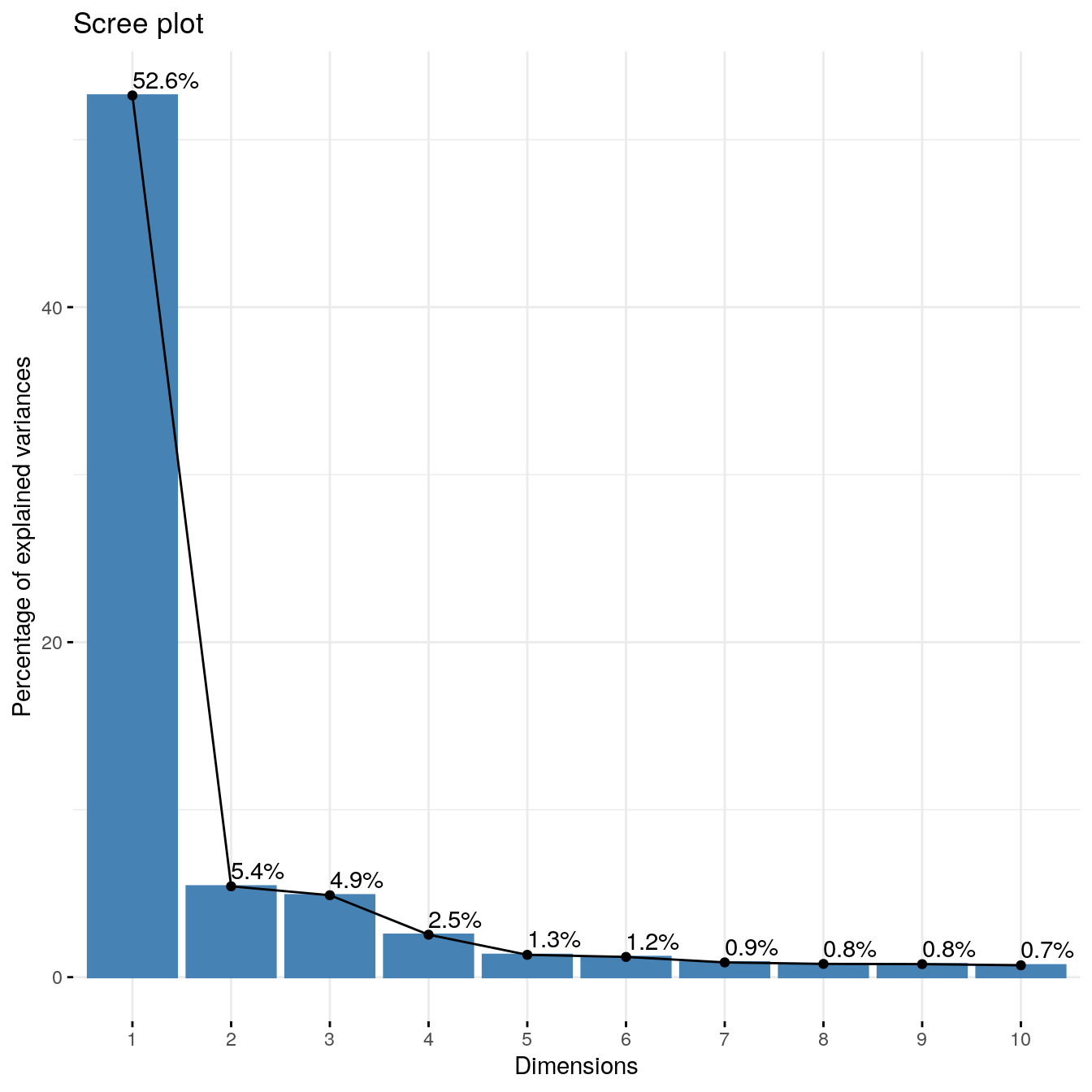
#fviz_eig(coex.pca.genes, choice = "eigenvalue", addlabels=TRUE)Hierarchical clustering
hc.norm = hclust(dist(g.space), method = "ward.D2")

dend <- as.dendrogram(hc.norm)

pca_1 = as.data.frame(coex.pca.genes$rotation[,1:10])
pca_1 = pca_1[order.dendrogram(dend),]

cut = cutree(hc.norm, k = 7, order_clusters_as_data = F)

#- Next lines are only to color and plot the secondary markers

tmp = get.pval(object = objE17,gene.set.col =unlist(layers),gene.set.row = colnames(g.space))
#>      L11      L12    L2/31    L2/32      L41      L42    L5/61    L5/62
#>   "Reln"   "Lhx5"  "Satb2"   "Cux1"   "Rorb"   "Sox5" "Bcl11b"  "Fezf2"
#>    Prog1    Prog2
#>    "Vim"   "Hes1"
#> [1] "Get p-values on a set of genes on columns on a set of genes on rows"
#> [1] "Using function S"
#> [1] "function to generate S "
for (m in unlist(layers)) {
  tmp = as.data.frame(tmp[order(tmp[,m]),])
  tmp$rank = c(1:nrow(tmp))
  colnames(tmp)[ncol(tmp)] = paste("rank",m,sep = ".")
  }
rank.genes = tmp[,(length(unlist(layers))+1):ncol(tmp)]
for (c in c(1:length(colnames(rank.genes)))) {
  colnames(rank.genes)[c] =strsplit(colnames(rank.genes)[c], split='.',fixed = T)[[1]][2]
}

L1 = rowSums(rank.genes[,layers[[1]]])
L1[layers[[1]]] = 1
L2 = rowSums(rank.genes[,layers[[2]]])
L2[layers[[2]]] = 1
L4 = rowSums(rank.genes[,layers[[3]]])
L4[layers[[3]]] = 1
L5 =rowSums(rank.genes[,layers[[4]]])
L5[layers[[4]]] = 1
P = rowSums(rank.genes[,layers[[5]]])
P[layers[[5]]] = 1
col.secondary = merge(L1,L2,by="row.names",all.x=TRUE)
colnames(col.secondary)[2:3] = c("L1","L2")
rownames(col.secondary) = col.secondary$Row.names
col.secondary = col.secondary[,2:ncol(col.secondary)]
col.secondary = merge(col.secondary,L4,by="row.names",all.x=TRUE)
colnames(col.secondary)[ncol(col.secondary)] = "L4"
rownames(col.secondary) = col.secondary$Row.names
col.secondary = col.secondary[,2:ncol(col.secondary)]
col.secondary = merge(col.secondary,L5,by="row.names",all.x=TRUE)
colnames(col.secondary)[ncol(col.secondary)] = "L5"
rownames(col.secondary) = col.secondary$Row.names
col.secondary = col.secondary[,2:ncol(col.secondary)]
col.secondary = merge(col.secondary,P,by="row.names",all.x=TRUE)
colnames(col.secondary)[ncol(col.secondary)] = "P"
rownames(col.secondary) = col.secondary$Row.names
col.secondary = col.secondary[,2:ncol(col.secondary)]

#  this part is to check that we will color as secondary markers only the genes linked to the
# primary with positive coex
temp.coex = as.matrix(objE17@coex[rownames(objE17@coex) %in% rownames(col.secondary),
                          colnames(objE17@coex) %in% unlist(layers)])
for (n in rownames(col.secondary)) {
  if(any(temp.coex[n,c("Reln","Lhx5")] < 0)){
    col.secondary[n,"L1"] = 100000
  }
  if(any(temp.coex[n,c("Cux1","Satb2")] < 0)){
    col.secondary[n,"L2"] = 100000
  }
  if(any(temp.coex[n,c("Rorb","Sox5")] < 0)){
    col.secondary[n,"L4"] = 100000
  }
  if(any(temp.coex[n,c("Bcl11b","Fezf2")] < 0)){
    col.secondary[n,"L5"] = 100000
  }
  if(any(temp.coex[n,c("Vim","Hes1")] < 0)){
    col.secondary[n,"P"] = 100000
  }
}

mylist.names <- c("L1", "L2", "L4","L5","P")
pos.link  <- vector("list", length(mylist.names))
names(pos.link) <- mylist.names
for (g in rownames(col.secondary)) {
  if(length( which(col.secondary[g,] == min(col.secondary[g,]))) == 1 ){
  pos.link[[which(col.secondary[g,] == min(col.secondary[g,])) ]] =
    c(pos.link[[which(col.secondary[g,] == min(col.secondary[g,])) ]], g)
  }
}
# ----


pca_1$highlight = with(pca_1,
          ifelse(rownames(pca_1) %in% pos.link$L5, "genes related to L5/6",
          ifelse(rownames(pca_1) %in% pos.link$L2 , "genes related to L2/3",
          ifelse(rownames(pca_1) %in% pos.link$P , "genes related to Prog" ,
          ifelse(rownames(pca_1) %in% pos.link$L1 , "genes related to L1" ,
          ifelse(rownames(pca_1) %in% pos.link$L4 ,"genes related to L4" ,
      "not marked"))))))

# But sort them based on their order in dend:
#colors_to_use <- pca_1$highlight[order.dendrogram(dend)]

#mycolours <- c("genes related to L5/6" = "#3C5488FF","genes related to L2/3"="#F39B7FFF","genes related to Prog"="#4DBBD5FF","genes related to L1"="#E64B35FF","genes related to L4" = "#91D1C2FF", "not marked"="#B09C85FF")
pca_1$hclust = cut

pca_1$colors = NA
pca_1[pca_1$highlight == "genes related to L5/6", "colors"] = "#3C5488FF"
pca_1[pca_1$highlight == "genes related to L2/3","colors"] = "#F39B7FFF"
pca_1[pca_1$highlight == "genes related to Prog","colors"] = "#4DBBD5FF"
pca_1[pca_1$highlight == "genes related to L1","colors"] = "#E64B35FF"
pca_1[pca_1$highlight == "genes related to L4","colors"] = "#91D1C2FF"
pca_1[pca_1$highlight == "not marked","colors"] = "#B09C85FF"


dend =branches_color(dend,k=7,col=c("#4DBBD5FF","#91D1C2FF","#E64B35FF","gray80","#3C5488FF","#F39B7FFF","gray80" ),groupLabels = T)
dend =color_labels(dend,k=7,labels = rownames(pca_1),col=pca_1$colors)


dend %>%
  dendextend::set("labels", ifelse(labels(dend) %in% rownames(pca_1)[rownames(pca_1) %in% colnames(g.space)] ,labels(dend),"")) %>%
  #  set("branches_k_color", value = c("gray80","#4DBBD5FF","#91D1C2FF" ,"gray80","#F39B7FFF","#E64B35FF","#3C5488FF"), k = 7) %>%
 plot(horiz=F, axes=T,ylim = c(0,80))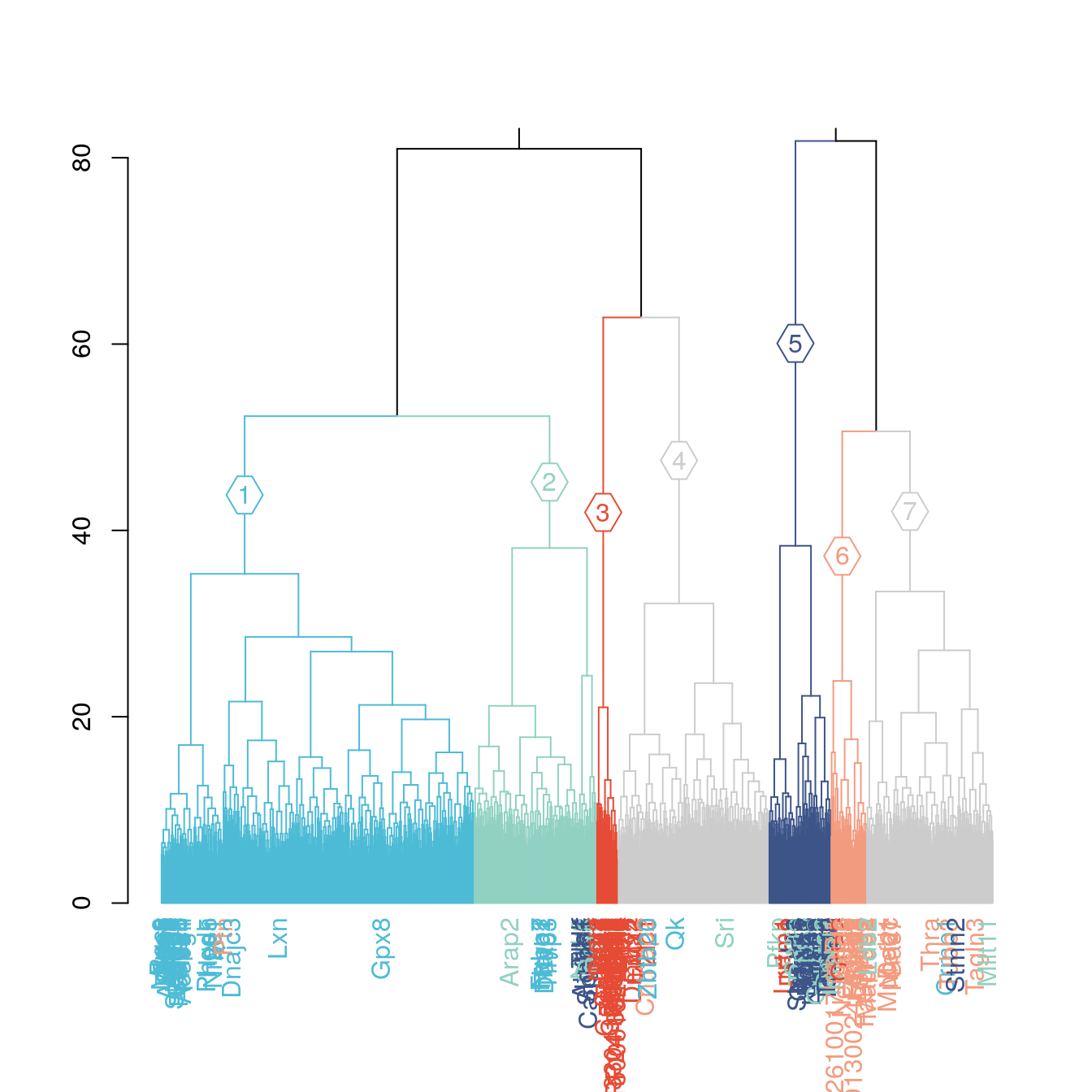
cluster = cut
cluster[cluster == 1] = "#4DBBD5FF"
cluster[cluster == 2] = "#91D1C2FF"
cluster[cluster == 3] =  "#E64B35FF"
cluster[cluster == 4] = "#B09C85FF"
cluster[cluster == 5] = "#3C5488FF"
cluster[cluster == 6] = "#F39B7FFF"
cluster[cluster == 7] = "#B09C85FF"


plot.new()
plot(dend,horiz=T, axes=T,xlim = c(100,0),leaflab = "none")
abline(v = 47, lty = 2)
colored_bars(cluster,dend,horiz = T,sort_by_labels_order = F,y_shift = 1,
               rowLabels= "" )
gridGraphics::grid.echo()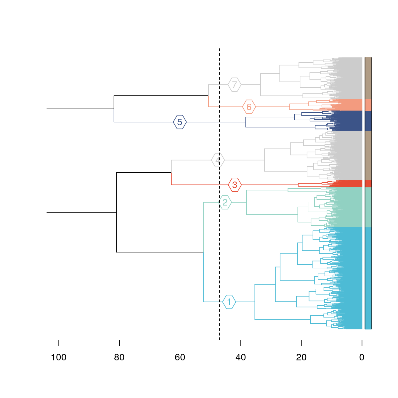
tree <- grid.grab()
par_pca = pca_1[colnames(g.space)[colnames(g.space) %in% rownames(pca_1)],]
#plot N 1
p1 <- ggparagraph(text = paste0(rownames(par_pca[par_pca$hclust == par_pca["Fezf2","hclust"],]), collapse = ", "),
                  face = "italic",
                  size =10,
                  color = "#3C5488FF")

#plot N 2
p2 = ggparagraph(text = paste0(rownames(par_pca[par_pca$hclust == unique(par_pca$hclust)[!unique(par_pca$hclust) %in% unique(par_pca[unlist(layers),"hclust"])][1],]), collapse = ", "),
                 face = "italic",
                 size =10,
                 color = "gray")

#plot N 3
p3 = ggparagraph(text = paste0(rownames(par_pca[par_pca$hclust == unique(par_pca$hclust)[!unique(par_pca$hclust) %in% unique(par_pca[unlist(layers),"hclust"])][2],]), collapse = ", "),
                 face = "italic",
                 size =10,
                 color = "gray")
#plot N 4
p4 = ggparagraph(text = paste0(rownames(par_pca[par_pca$hclust == par_pca["Reln","hclust"],]), collapse = ", "),
                 face = "italic",
                 size =10,
                 color = "#E64B35FF")

#plot N 5
p5 = ggparagraph(text = paste0(rownames(par_pca[par_pca$hclust == par_pca["Cux1","hclust"],]), collapse = ", "),
                 face = "italic",
                 size =10,
                 color = par_pca["Cux1","colors"])
#plot N 6
p6 = ggparagraph(text = paste0(rownames(par_pca[par_pca$hclust == par_pca["Rorb","hclust"],]), collapse = ", "),
                 face = "italic",
                 size =10,
                 color = par_pca["Rorb","colors"])
#plot N 7
p7 = ggparagraph(text = paste0(rownames(par_pca[par_pca$hclust == par_pca["Vim","hclust"],]), collapse = ", "),
                 face = "italic",
                 size =10,
                 color = par_pca["Vim","colors"])

w = ggparagraph(text = " ",
                 face = "italic",
                 size =10,
                 color = "white")

pp =ggarrange(p3,p5,p1,p2,p4,p6,p7,w,
          ncol = 1, nrow = 8,
          heights = c(0.1,0.15,0.23, 0.1, 0.2, 0.2, 0.1, 0.35))


lay <- rbind(c(1,NA),
             c(1,2.5),
             c(1,2.5),
             c(1,2.5),
             c(1,2.5),
             c(1,2.5),
             c(1,NA))

gridExtra::grid.arrange(tree, pp, layout_matrix = lay)
or just with primary markers
# some more genes as landmarks
controls =list("genes related to L5/6"=c("Foxp2","Tbr1"), "genes related to L2/3"=c("Mef2c"), "genes related to Prog"=c("Nes","Sox2") , "genes related to L1"=c() , "genes related to L4"=c())
dend %>%
dendextend::set("labels", ifelse(labels(dend) %in% rownames(pca_1)[rownames(pca_1) %in% c(unlist(layers),unlist(controls))], labels(dend), "")) %>%
  dendextend::set("branches_k_color", value = c("gray80","#4DBBD5FF","#91D1C2FF" ,"gray80","#F39B7FFF","#E64B35FF","#3C5488FF"), k = 7) %>%
plot(horiz=F, axes=T,ylim = c(0,100))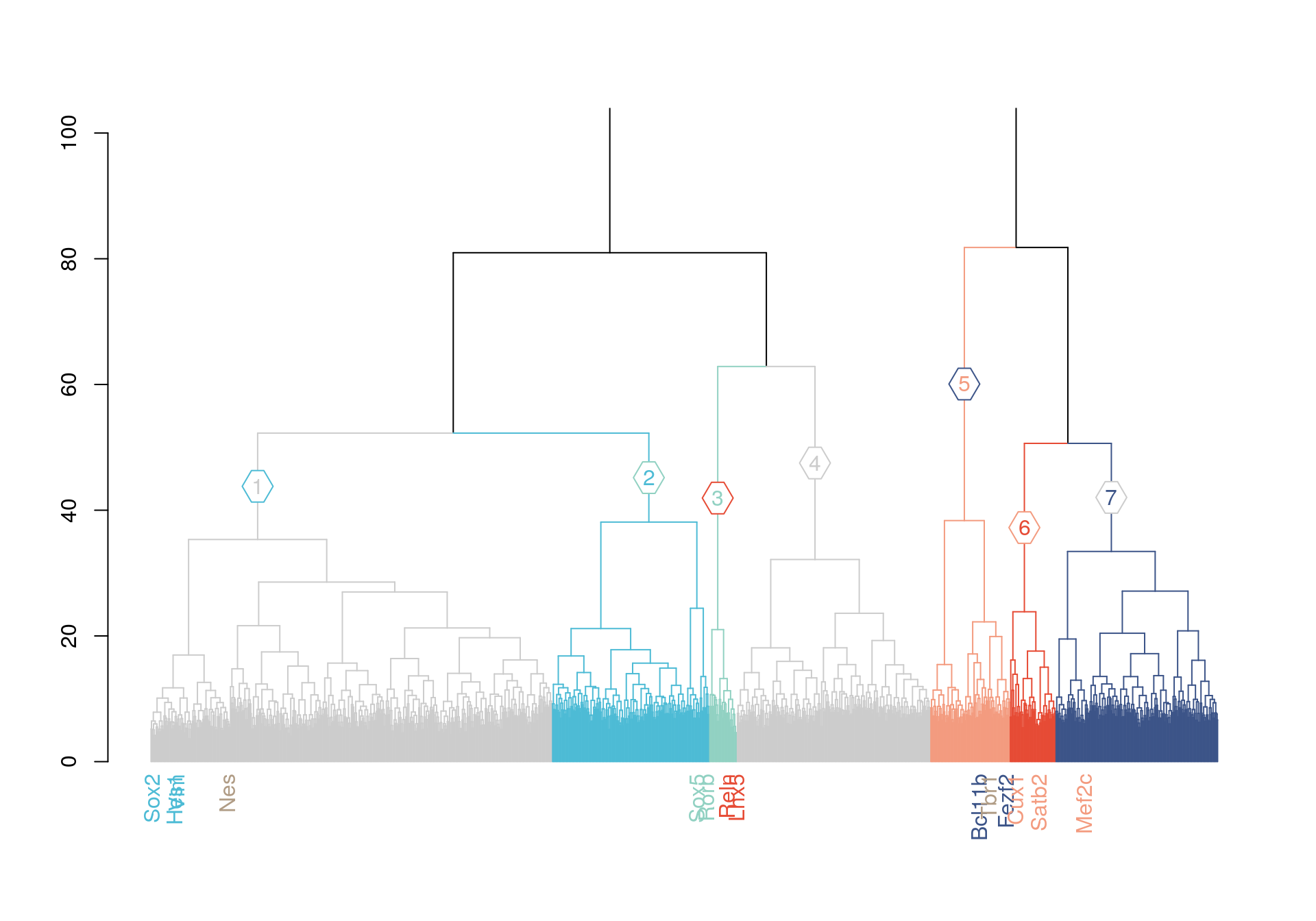
Now we can plot the PCA
# dataframe to be able to label only primary markers and control genes
textdf <- pca_1[rownames(pca_1) %in% c(unlist(layers),unlist(controls)) , ]

 for (m in c(1:length(controls))) {
  for (g in controls[[m]]) {
    if(g %in% rownames(textdf)){
      textdf[g,"highlight"] = names(controls[m])
    }
  }
}

# deciding the colors
mycolours <- c("genes related to L5/6" = "#3C5488FF","genes related to L2/3"="#F39B7FFF","genes related to Prog"="#4DBBD5FF","genes related to L1"="#E64B35FF","genes related to L4" = "#91D1C2FF", "not marked"="#B09C85FF")

# to assing correcly the cluster number and the color
mycolours2 = c("Reln","Satb2","Rorb","Bcl11b","Vim")
names(mycolours2) = unique(cut[unlist(layers)])

mycolours2[mycolours2 == "Reln"] = "#E64B35FF"
mycolours2[mycolours2 == "Satb2"] = "#F39B7FFF"
mycolours2[mycolours2 == "Rorb"] = "#91D1C2FF"
mycolours2[mycolours2 == "Bcl11b"] = "#3C5488FF"
mycolours2[mycolours2 == "Vim"] = "#4DBBD5FF"
color_to_add = unique(pca_1$hclust)[!unique(pca_1$hclust) %in% as.numeric(names(mycolours2))]
names(color_to_add) = unique(pca_1$hclust)[!unique(pca_1$hclust) %in% as.numeric(names(mycolours2))]
color_to_add[color_to_add %in%
                 unique(pca_1$hclust)[!unique(pca_1$hclust) %in% as.numeric(names(mycolours2))]] = "#B09C85FF"
mycolours2 = c(mycolours2,color_to_add)

pca1 = ggplot(subset(pca_1,!hclust %in% unique(cut[unlist(layers)])  ), aes(x=PC1, y=PC2)) +  geom_point(alpha = 0.3,color = "#B09C85FF",size=1)

pca_1$names = rownames(pca_1)
#pca2 = pca1 + geom_point(data = subset(pca_1, highlight != "not marked" ), aes(x=PC1, y=PC2, colour=hclust),size=2.5,alpha = 0.9)
pca2 = pca1 + geom_point(data = subset(pca_1, hclust %in% unique(cut[unlist(layers)]) ), aes(x=PC1, y=PC2, colour=as.character(hclust)),size=1,alpha = 0.5) +
 scale_color_manual( "Status", values = mycolours2)  +
  scale_fill_manual( "Status", values = mycolours2)  +
  xlab("") + ylab("") +
  geom_label_repel(data =textdf , aes(x = PC1, y = PC2, label = rownames(textdf),fill=as.character(hclust)),
                   label.size = NA,
                   alpha = 0.5,
                   direction = "both",
                   na.rm=TRUE,
                   seed = 1234) +
  geom_label_repel(data =textdf , aes(x = PC1, y = PC2, label = rownames(textdf)),
                   label.size = NA,
                   segment.color = 'black',
                   segment.size = 0.5,
                   direction = "both",
                   alpha = 1,
                   na.rm=TRUE,
                   fill = NA,
                   seed = 1234) +
  ggtitle("PCA") +
  theme_light(base_size=10) +
    theme(axis.text.x=element_blank(),plot.title = element_text(size=14,
                                    face="italic",
                                    color="#3C5488FF",
                                    hjust=0.01,
                                    lineheight=1.2,margin = margin(t = 5, b = -15)),
        axis.text.y=element_blank(),
        legend.position = "none")  # titl)

pca2 #+ geom_encircle(data = pca_1, aes(group=hclust)) 
set.seed(NULL)
cell = sample(ncol(objE17@raw),1,replace = T)
print(cell)
#> [1] 461
genes.to.color.red = which(objE17@raw[,cell] > 0)
length(genes.to.color.red)
#> [1] 1199

pca3 = pca2 + geom_point(data = subset(pca_1, names %in% names(genes.to.color.red)), color="red")

pca3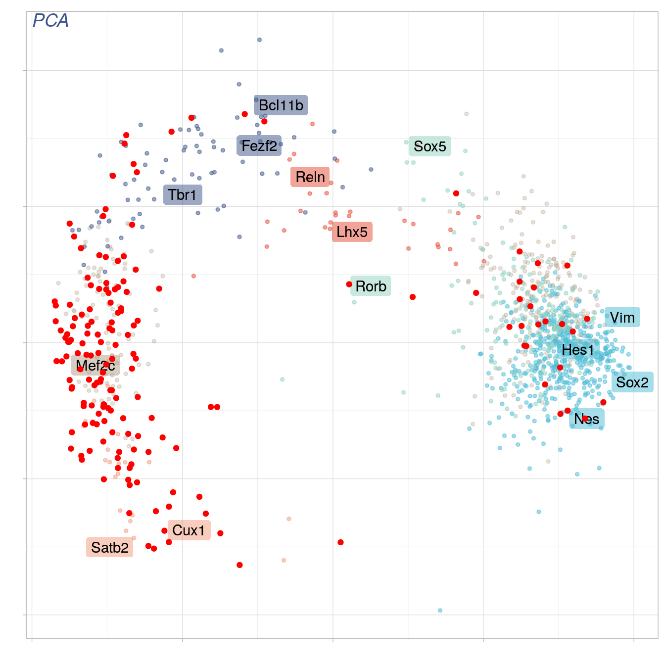
t-SNE code and plot
# run the t-SNE
cl.genes.tsne = Rtsne(g.space ,initial_dims = 100, dims = 2, perplexity=30,eta = 200, verbose=F, max_iter = 3000,theta=0.4,num_threads = 10,pca_center = T, pca_scale = FALSE, normalize = T )

d_tsne_1 = as.data.frame(cl.genes.tsne$Y)
rownames(d_tsne_1) = rownames(g.space)

d_tsne_1 = d_tsne_1[order.dendrogram(dend),]

# save the cluster numebr inside a dataframe with the t-SNE information
d_tsne_1$hclust = cut

d_tsne_1$names = rownames(d_tsne_1)

# as before to label only some genes
textdf <- d_tsne_1[rownames(d_tsne_1) %in% c(unlist(layers),unlist(controls)),]

for (m in c(1:length(controls))) {
  for (g in controls[[m]]) {
    if(g %in% rownames(textdf)){
      textdf[g,"highlight"] = names(controls[m])
    }
  }
}


 p1 = ggplot(subset(d_tsne_1,!hclust %in% unique(cut[unlist(layers)])), aes(x=V1, y=V2)) +  geom_point(alpha = 0.3, color = "#B09C85FF", size=1)

p2 = p1 + geom_point(data = subset(d_tsne_1, hclust %in% unique(cut[unlist(layers)]) ), aes(x=V1, y=V2, colour=as.character(hclust)),size=1,alpha = 0.5) +
    scale_color_manual("Status", values = mycolours2)  +
  scale_fill_manual("Status", values = mycolours2)  +
  xlab("") + ylab("")+
  geom_label_repel(data =textdf , aes(x = V1, y = V2, label = names,fill=as.character(hclust)),
                   label.size = NA,
                   alpha = 0.5,
                   direction = "both",
                   na.rm=TRUE,
                   seed = 1234) +
  geom_label_repel(data =textdf , aes(x = V1, y = V2, label = names),
                   label.size = NA,
                   segment.color = 'black',
                   segment.size = 0.5,
                   direction = "both",
                   alpha = 1,
                   na.rm=TRUE,
                   fill = NA,
                   seed = 1234) +
  ggtitle("t-SNE") +
  theme_light(base_size=10) +
  theme(axis.text.x=element_blank(),plot.title = element_text(size=14,
                                    face="italic",
                                    color="#3C5488FF",
                                    hjust=0.01,
                                    lineheight=1.2,margin = margin(t = 5, b = -15)),
        axis.text.y=element_blank(),
        legend.position = "none")  # titl)
p2
Code to create an iteractive plot. This can be modified to be used with all the plots.
p = ggplot(d_tsne_1, aes(x=V1, y=V2, text= paste("gene: ",names))) +
  geom_point(size=2, aes(colour=as.character(hclust)), alpha=0.8) +
  scale_color_manual("Status", values = mycolours2)  +
  xlab("") + ylab("") +
  ggtitle("t-SNE") +
  theme_light(base_size=10) +
  theme(axis.text.x=element_blank(),
        axis.text.y=element_blank())

ggplotly(p)
Multidimensional scaling (MDS) and plot
# run the MDS
genes.dist.euc =  dist(g.space, method =  "euclidean")
#fit <- isoMDS(genes.dist.euc) # not linear
fit <- isoMDS(genes.dist.euc)
#> initial  value 11.623631
#> final  value 9.513077
#> converged

fit.genes = as.data.frame(fit$points)

fit.genes = fit.genes[order.dendrogram(dend),]

fit.genes$hclust = cut


fit.genes$names = rownames(fit.genes)

mycolours3 <- c("cluster L5/6 markers" = "#3C5488FF","cluster L2/3 markers"="#F39B7FFF","cluster Prog markers"="#4DBBD5FF","cluster L1 markers"="#E64B35FF","cluster L4 markers" = "#91D1C2FF", "not identified cluster"="#B09C85FF")

#mycolours3 <- c("cluster layer V-VI markers" = "#3C5488FF","cluster layer II-III markers"="#F39B7FFF","cluster progenitor markers"="#4DBBD5FF","cluster layer I markers"="#E64B35FF","cluster layer IV markers" = "#91D1C2FF", "not identified cluster"="#B09C85FF")


#fit.genes$hclust = factor(cutree(hc.norm, 7))
used = vector()
for (k in c(1:length(layers))) {
  #print(k)
  tt =as.numeric(cut[layers[[k]]][1])
  fit.genes[fit.genes$hclust == tt,"cluster"] = paste("cluster",names(layers[k]),"markers", sep = " " )
  used = c(used,cut[layers[[k]]][1])
}

fit.genes[fit.genes$hclust %in% (unique(fit.genes$hclust)[!unique(fit.genes$hclust) %in% used]),]$cluster = "not identified cluster"

textdf <- fit.genes[rownames(fit.genes) %in% c(unlist(layers),unlist(controls)),]

   f1 = ggplot(subset(fit.genes,!hclust %in% unique(cut[unlist(layers)]) ), aes(x=V1, y=V2)) +  geom_point(alpha = 0.3, color = "#B09C85FF", size=1)

f2 = f1 + geom_point(data = subset(fit.genes, hclust %in% unique(cut[unlist(layers)]) ),
                     aes(x=V1, y=V2, colour=cluster), size=1,alpha = 0.5) +
  scale_color_manual("Status", values = mycolours3,
                     labels = c("Layer I cluster ","Layers II/III cluster",
                                "Layer IV cluster",
                                "Layers V/VI cluster",
                                "Progenitors cluster") )  +
  scale_fill_manual("Status", values = mycolours3)  +
  xlab("") + ylab("")+
  geom_label_repel(data =textdf , aes(x = V1, y = V2, label = rownames(textdf),fill=cluster),
                   label.size = NA,
                   alpha = 0.5,
                   direction ="both",
                   na.rm=TRUE,
                   seed = 1234, show.legend = FALSE) +
  geom_label_repel(data =textdf , aes(x = V1, y = V2, label = rownames(textdf)),
                   label.size = NA,
                   segment.color = 'black',
                   segment.size = 0.5,
                   direction = "both",
                   alpha = 1,
                   na.rm=TRUE,
                   fill = NA,
                   seed = 1234, show.legend = FALSE) +
  ggtitle("MDS") +
  theme_light(base_size=10) +
  theme(axis.text.x=element_blank(),plot.title = element_text(size=14,
                                    face="italic",
                                    color="#3C5488FF",
                                    hjust=0.01,
                                    lineheight=1.2,margin = margin(t = 5, b = -15)),
        axis.text.y=element_blank(),
        legend.title = element_blank(),
        legend.text = element_text(color = "#3C5488FF",face ="italic" ),
        legend.position = "bottom")  # titl)


f2 + scale_y_reverse()+ scale_x_reverse()#+ geom_encircle(data = fit.genes, aes(group=`5_clusters`)) 
sessionInfo()
#> R version 4.1.2 (2021-11-01)
#> Platform: x86_64-pc-linux-gnu (64-bit)
#> Running under: Ubuntu 18.04.6 LTS
#>
#> Matrix products: default
#> BLAS:   /usr/lib/x86_64-linux-gnu/openblas/libblas.so.3
#> LAPACK: /usr/lib/x86_64-linux-gnu/libopenblasp-r0.2.20.so
#>
#> locale:
#>  [1] LC_CTYPE=en_US.UTF-8       LC_NUMERIC=C
#>  [3] LC_TIME=en_US.UTF-8        LC_COLLATE=en_US.UTF-8
#>  [5] LC_MONETARY=en_US.UTF-8    LC_MESSAGES=en_US.UTF-8
#>  [7] LC_PAPER=en_US.UTF-8       LC_NAME=C
#>  [9] LC_ADDRESS=C               LC_TELEPHONE=C
#> [11] LC_MEASUREMENT=en_US.UTF-8 LC_IDENTIFICATION=C
#>
#> attached base packages:
#> [1] grid      stats     graphics  grDevices utils     datasets  methods
#> [8] base
#>
#> other attached packages:
#>  [1] ggpubr_0.4.0      dendextend_1.15.1 MASS_7.3-54       htmlwidgets_1.5.3
#>  [5] forcats_0.5.1     stringr_1.4.0     dplyr_1.0.6       purrr_0.3.4
#>  [9] readr_1.4.0       tidyr_1.1.3       tibble_3.1.2      tidyverse_1.3.1
#> [13] plotly_4.9.3      Rtsne_0.15        ggrepel_0.9.1     COTAN_0.99.7
#> [17] factoextra_1.0.7  ggplot2_3.3.3
#>
#> loaded via a namespace (and not attached):
#>  [1] colorspace_2.0-1     ggsignif_0.6.1       rjson_0.2.20
#>  [4] ellipsis_0.3.2       rio_0.5.26           circlize_0.4.12
#>  [7] GlobalOptions_0.1.2  fs_1.5.0             clue_0.3-59
#> [10] rstudioapi_0.13      farver_2.1.0         fansi_0.4.2
#> [13] lubridate_1.7.10     xml2_1.3.2           codetools_0.2-18
#> [16] doParallel_1.0.16    knitr_1.33           jsonlite_1.7.2
#> [19] Cairo_1.5-12.2       broom_0.7.6          cluster_2.1.2
#> [22] dbplyr_2.1.1         png_0.1-7            compiler_4.1.2
#> [25] httr_1.4.2           basilisk_1.5.0       backports_1.2.1
#> [28] assertthat_0.2.1     Matrix_1.4-0         lazyeval_0.2.2
#> [31] cli_2.5.0            htmltools_0.5.1.1    tools_4.1.2
#> [34] gtable_0.3.0         glue_1.4.2           Rcpp_1.0.6
#> [37] carData_3.0-4        cellranger_1.1.0     jquerylib_0.1.4
#> [40] vctrs_0.3.8          crosstalk_1.1.1      iterators_1.0.13
#> [43] xfun_0.23            openxlsx_4.2.3       rvest_1.0.0
#> [46] lifecycle_1.0.0      rstatix_0.7.0        scales_1.1.1
#> [49] basilisk.utils_1.5.0 hms_1.1.0            parallel_4.1.2
#> [52] RColorBrewer_1.1-2   ComplexHeatmap_2.9.0 yaml_2.2.1
#> [55] curl_4.3.1           reticulate_1.20      gridExtra_2.3
#> [58] stringi_1.6.2        highr_0.9            S4Vectors_0.31.0
#> [61] foreach_1.5.1        BiocGenerics_0.39.0  filelock_1.0.2
#> [64] zip_2.1.1            shape_1.4.6          rlang_0.4.11
#> [67] pkgconfig_2.0.3      matrixStats_0.58.0   evaluate_0.14
#> [70] lattice_0.20-45      labeling_0.4.2       cowplot_1.1.1
#> [73] tidyselect_1.1.1     magrittr_2.0.1       R6_2.5.0
#> [76] IRanges_2.27.0       generics_0.1.0       DBI_1.1.1
#> [79] pillar_1.6.1         haven_2.4.1          foreign_0.8-81
#> [82] withr_2.4.2          abind_1.4-5          dir.expiry_1.1.0
#> [85] modelr_0.1.8         crayon_1.4.1         car_3.0-10
#> [88] utf8_1.2.1           rmarkdown_2.11       viridis_0.6.1
#> [91] GetoptLong_1.0.5     readxl_1.3.1         data.table_1.14.0
#> [94] reprex_2.0.0         digest_0.6.27        gridGraphics_0.5-1
#> [97] stats4_4.1.2         munsell_0.5.0        viridisLite_0.4.0