E15.5 cortex
library(COTAN)
library(data.table)
library(Matrix)
library(ggrepel)
#> Loading required package: ggplot2
mycolours <- c(A = "#8491B4B2", B = "#E64B35FF")
my_theme = theme(axis.text.x = element_text(size = 14,
angle = 0, hjust = 0.5, vjust = 0.5,
face = "plain", colour = "#3C5488FF"),
axis.text.y = element_text(size = 14,
angle = 0, hjust = 0, vjust = 0.5,
face = "plain", colour = "#3C5488FF"),
axis.title.x = element_text(size = 14,
angle = 0, hjust = 0.5, vjust = 0,
face = "plain", colour = "#3C5488FF"),
axis.title.y = element_text(size = 14,
angle = 90, hjust = 0.5, vjust = 0.5,
face = "plain", colour = "#3C5488FF"))data = as.data.frame(fread(paste(data_dir,
"GSE107122_E155_Combined_Only_Cortical_Cells_DGE.txt.gz",
sep = "/")))
data = as.data.frame(data)
rownames(data) = data$V1
data = data[, 2:ncol(data)]
data[1:10, 1:10]
#> CTGATGGTCTTT CACCGTTAGGAC TAATTCATTCTC TGAGATTATCTT CCCGGCGGCCAC
#> 0610005C13Rik 0 0 0 0 0
#> 0610007N19Rik 0 0 1 0 3
#> 0610007P14Rik 0 1 0 2 1
#> 0610009B22Rik 2 1 0 0 1
#> 0610009D07Rik 4 1 0 3 4
#> 0610009E02Rik 0 0 0 0 0
#> 0610009L18Rik 0 0 0 0 0
#> 0610009O20Rik 1 0 0 0 0
#> 0610010F05Rik 0 5 2 2 0
#> 0610010K14Rik 0 0 0 0 0
#> GTCCTTCCATGT AGCTCGTTTCCA CATATCCATCGC TTACCTTCTCTG ACCTCTCACTTA
#> 0610005C13Rik 0 0 0 0 0
#> 0610007N19Rik 0 0 0 0 0
#> 0610007P14Rik 1 1 3 0 0
#> 0610009B22Rik 0 0 0 0 2
#> 0610009D07Rik 2 3 0 7 2
#> 0610009E02Rik 0 0 0 0 0
#> 0610009L18Rik 1 0 0 0 1
#> 0610009O20Rik 0 0 0 0 0
#> 0610010F05Rik 0 2 0 1 2
#> 0610010K14Rik 0 0 0 0 0Define a directory where the ouput will be stored.
1 Analytical pipeline
Initialize the COTAN object with the row count table and the metadata for the experiment.
obj = new("scCOTAN", raw = data)
obj = initRaw(obj, GEO = "GSE107122", sc.method = "DropSeq",
    cond = "mouse cortex E15.5")
#> [1] "Initializing S4 object"
Now we can start the cleaning. Analysis requires and starts from a matrix of raw UMI counts after removing possible cell doublets or multiplets and low quality or dying cells (with too high mtRNA percentage, easily done with Seurat or other tools).
If we do not want to consider the mitochondrial genes we can remove them before starting the analysis.
genes_to_rem = rownames(obj@raw[grep("^mt",
    rownames(obj@raw)), ])  #genes to remove : mithocondrial
obj@raw = obj@raw[!rownames(obj@raw) %in%
    genes_to_rem, ]
cells_to_rem = colnames(obj@raw[which(colSums(obj@raw) ==
    0)])
obj@raw = obj@raw[, !colnames(obj@raw) %in%
    cells_to_rem]
We want also to define a prefix to identify the sample.
t = "E15_cortex_clean"

print(paste("Condition ", t, sep = ""))
#> [1] "Condition E15_cortex_clean"
#--------------------------------------
n_cells = length(colnames(obj@raw))
print(paste("n cells", n_cells, sep = " "))
#> [1] "n cells 2955"

n_it = 1

# obj@raw = obj@raw[rownames(cells),
# colnames(cells)]
2 Data cleaning
First, we create the directory to store all information regarding the data cleaning.
if (!file.exists(out_dir)) {
    dir.create(file.path(out_dir))
}

if (!file.exists(paste(out_dir, "cleaning",
    sep = ""))) {
    dir.create(file.path(out_dir, "cleaning"))
}
ttm = clean(obj)
#> [1] "Start estimation mu with linear method"
#> [1] 12889 2955
#> rowname AATGCGGACAGG TTCTAAACTTCC TCTTCCCGACGA
#> 5373 Hbb-bs 533.027446 177.779161 274.830198
#> 5372 Hba-a1 142.140652 80.808710 194.782567
#> 5374 Hbb-bt 160.618937 19.394090 24.014289
#> 11759 Tuba1a 5.685626 35.555832 32.019052
#> 11429 Tmsb4x 1.421407 45.252877 13.341272
#> 6514 Malat1 11.371252 22.626439 8.004763
#> 5543 Hnrnpa2b1 5.685626 19.394090 16.009526
#> 9599 Rps5 9.949846 16.161742 8.004763
#> 9517 Rpl32 8.528439 6.464697 16.009526
#> 7448 Nfib 2.842813 19.394090 5.336509
#> 11425 Tmsb10 1.421407 25.858787 0.000000
#> 9487 Rpl13a 9.949846 16.161742 0.000000
#> 11724 Ttc3 2.842813 19.394090 2.668254
#> 7433 Neurod6 0.000000 16.161742 8.004763
#> 5708 Igfbpl1 2.842813 6.464697 13.341272
obj = ttm$object
ttm$pca.cell.2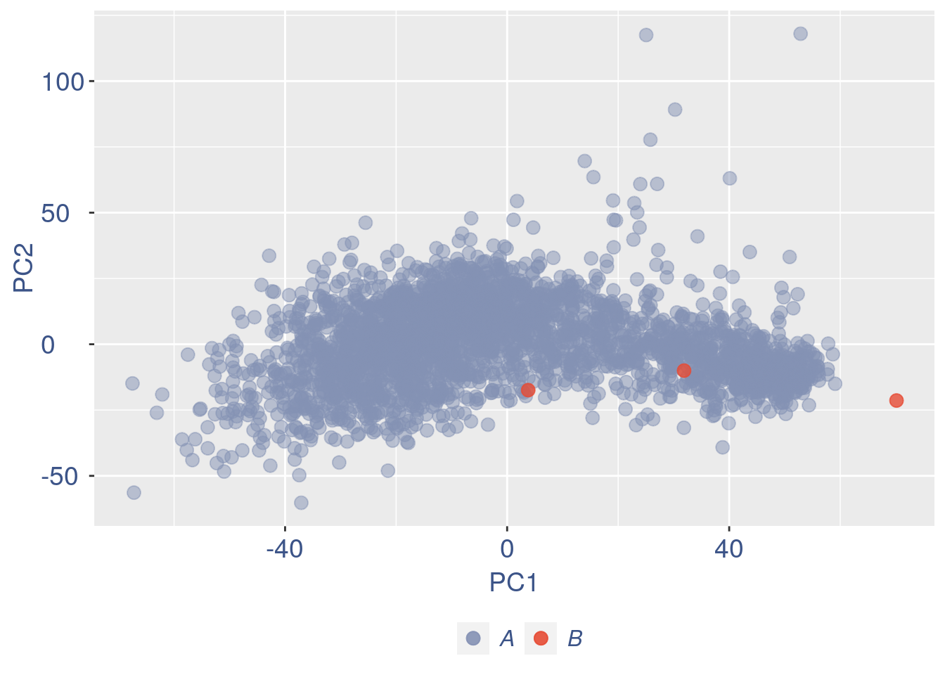
Run this when B cells need to be removed.
pdf(paste(out_dir, "cleaning/", t, "_", n_it,
    "_plots_before_cells_exlusion.pdf", sep = ""))
ttm$pca.cell.2
ggplot(ttm$D, aes(x = n, y = means)) + geom_point() +
    geom_text_repel(data = subset(ttm$D,
        n > (max(ttm$D$n) - 15)), aes(n,
        means, label = rownames(ttm$D[ttm$D$n >
            (max(ttm$D$n) - 15), ])), nudge_y = 0.05,
        nudge_x = 0.05, direction = "x",
        angle = 90, vjust = 0, segment.size = 0.2) +
    ggtitle("B cell group genes mean expression") +
    my_theme + theme(plot.title = element_text(color = "#3C5488FF",
    size = 20, face = "italic", vjust = -5,
    hjust = 0.02))
dev.off()
#> png
#>   2

if (length(ttm$cl1) < length(ttm$cl2)) {
    to_rem = ttm$cl1
} else {
    to_rem = ttm$cl2
}
n_it = n_it + 1
obj@raw = obj@raw[, !colnames(obj@raw) %in%
    to_rem]
# obj@raw = obj@raw[rownames(obj@raw)
# %in% rownames(cells),colnames(obj@raw)
# %in% colnames(cells)]
gc()
#>             used   (Mb) gc trigger   (Mb)  max used   (Mb)
#> Ncells   3742647  199.9    6026262  321.9   6026262  321.9
#> Vcells 256234246 1955.0  382282220 2916.6 318501784 2430.0

ttm = clean(obj)
#> [1] "Start estimation mu with linear method"
#> [1] 12887  2952
#>        rowname GTGTCGGCGCTN TTACGCACATCT TATTGGCCCATC
#> 6512    Malat1   180.232409   213.042519   234.198856
#> 11757   Tuba1a    28.776603    19.367502    12.774483
#> 10534     Sox4     6.058232    41.501789    12.774483
#> 7532      Nnat     4.543674    41.501789     8.516322
#> 6730      Meg3     1.514558    38.735003     0.000000
#> 7446      Nfib     7.572790    27.667860     4.258161
#> 7431   Neurod6     9.087348    13.833930    12.774483
#> 11165     Tia1     4.543674     0.000000    29.807127
#> 5606  Hsp90ab1    13.631022     5.533572     8.516322
#> 11427   Tmsb4x     9.087348    16.600716     0.000000
#> 7509      Nktr     0.000000    16.600716     8.516322
#> 5225     Gria2    16.660139     2.766786     4.258161
#> 9978    Sfrs18    12.116464     2.766786     8.516322
#> 11047     Tcf4    10.601906     0.000000    12.774483
#> 671       Actb     9.087348    13.833930     0.000000
# ttm = clean.sqrt(obj, cells)
obj = ttm$object

ttm$pca.cell.2
#> png
#>   2
#>             used   (Mb) gc trigger   (Mb)  max used   (Mb)
#> Ncells   3742887  199.9    6026262  321.9   6026262  321.9
#> Vcells 263308011 2008.9  660874875 5042.1 660872768 5042.1
#> [1] "Start estimation mu with linear method"
#> [1] 12885  2949
#>         rowname TATCATGGTGCC GGCGACCTGCCA CATGTCAAAGGC GTTAGGCCCCAC
#> 3762      Fabp7    81.548823   79.2452455   121.248711    80.032947
#> 2916        Dbi    30.166435   18.9971479    30.312178    20.992248
#> 6511     Malat1     8.287482    5.4277565     3.637461    22.304264
#> 11425    Tmsb4x    15.580466   35.2804175    14.549845     7.872093
#> 11755    Tuba1a    15.248967   26.0532314    21.824768    11.808140
#> 8858        Ptn    13.259971    8.6844105     0.000000    44.608528
#> 671        Actb    11.270976   17.9115966     7.274923     6.560078
#> 7089        Mt3    11.270976   11.9410644    20.612281     6.560078
#> 8113     Pea15a     8.950481    5.4277565     9.699897     3.936047
#> 902       Aldoc     4.309491    3.2566539     9.699897     9.184109
#> 2383        Ckb     8.618981    5.4277565     7.274923     6.560078
#> 5605   Hsp90ab1     9.944978    5.4277565     9.699897     6.560078
#> 11751     Ttyh1     5.303989    3.2566539    12.124871    15.744186
#> 1089       Apoe     4.309491    0.5427757     0.000000    39.360466
#> 5540  Hnrnpa2b1     6.298486    6.5133078     2.424974     5.248062
#>       ATTTGAGCACGC GCGCCCTTTCCA CGCTAGTTTCGG CCCCATCAGTCG ATCTTTCAGTCG
#> 3762    128.944886   145.410225   79.5134242    79.616006    59.889472
#> 2916     29.756512    30.420549   28.6618157    25.141897    19.963157
#> 6511     16.531396    27.986905   17.5669193    21.789644    73.198244
#> 11425    23.143954    21.902795   14.7931952    20.951580    24.953947
#> 11755    19.837675    20.685974   23.1143675    14.247075    14.972368
#> 8858     23.143954    12.776631   14.7931952    15.923201    13.308772
#> 671       1.653140    14.601864   16.6423446     8.380632     8.317982
#> 7089      6.612558    12.168220    9.2457470     2.514190     3.327193
#> 8113      8.265698    10.342987   10.1703217    11.732885     4.990789
#> 902      11.571977     8.517754    2.7737241     4.190316    11.645175
#> 2383      8.265698    10.951398    6.4720229     6.704506     1.663596
#> 5605     11.571977     4.867288    3.6982988     7.542569     4.990789
#> 11751     9.918837     4.867288    3.6982988     6.704506     0.000000
#> 1089      3.306279     1.825233    0.9245747     2.514190     9.981579
#> 5540      8.265698     9.126165    5.5474482    10.056759     9.981579
#>       TTGTGAAGGATC
#> 3762     99.645146
#> 2916     25.185037
#> 6511      7.665011
#> 11425    17.520026
#> 11755    13.140019
#> 8858      9.855014
#> 671      14.235021
#> 7089      7.665011
#> 8113      7.665011
#> 902       7.665011
#> 2383      8.760013
#> 5605      4.380006
#> 11751     6.570010
#> 1089      4.380006
#> 5540      3.285005
Run this only in the last iteration, instead the previous code, when B cells group has not to be removed.
pdf(paste(out_dir, "cleaning/", t, "_", n_it,
    "_plots_before_cells_exlusion.pdf", sep = ""))
ttm$pca.cell.2
ggplot(ttm$D, aes(x = n, y = means)) + geom_point() +
    geom_text_repel(data = subset(ttm$D,
        n > (max(ttm$D$n) - 15)), aes(n,
        means, label = rownames(ttm$D[ttm$D$n >
            (max(ttm$D$n) - 15), ])), nudge_y = 0.05,
        nudge_x = 0.05, direction = "x",
        angle = 90, vjust = 0, segment.size = 0.2) +
    ggtitle(label = "B cell group genes mean expression",
        subtitle = " - B group NOT removed -") +
    my_theme + theme(plot.title = element_text(color = "#3C5488FF",
    size = 20, face = "italic", vjust = -10,
    hjust = 0.02), plot.subtitle = element_text(color = "darkred",
    vjust = -15, hjust = 0.01))

dev.off()
#> png
#>   2
To colour the pca based on nu_j (so the cells’ efficiency).
nu_est = round(obj@nu, digits = 7)

plot.nu <- ggplot(ttm$pca_cells, aes(x = PC1,
    y = PC2, colour = log(nu_est)))

plot.nu = plot.nu + geom_point(size = 1,
    alpha = 0.8) + scale_color_gradient2(low = "#E64B35B2",
    mid = "#4DBBD5B2", high = "#3C5488B2",
    midpoint = log(mean(nu_est)), name = "ln (nu)") +
    ggtitle("Cells PCA coloured by cells efficiency") +
    my_theme + theme(plot.title = element_text(color = "#3C5488FF",
    size = 20), legend.title = element_text(color = "#3C5488FF",
    size = 14, face = "italic"), legend.text = element_text(color = "#3C5488FF",
    size = 13), legend.key.width = unit(2,
    "mm"), legend.position = "right")

pdf(paste(out_dir, "cleaning/", t, "_plots_PCA_efficiency_colored.pdf",
    sep = ""))
plot.nu
dev.off()
#> png
#>   2

plot.nu
The next part is use to remove the cells with efficiency too low.
nu_df = data.frame(nu = sort(obj@nu), n = c(1:length(obj@nu)))

ggplot(nu_df, aes(x = n, y = nu)) + geom_point(colour = "#8491B4B2",
    size = 1) + my_theme  #+ ylim(0,1) + xlim(0,70)
We can zoom on the smallest values and, if we detect a clear elbow, we can decide to remove the cells.
yset = 0.28  #threshold to remove low UDE cells
plot.ude <- ggplot(nu_df, aes(x = n, y = nu)) +
    geom_point(colour = "#8491B4B2", size = 1) +
    my_theme + ylim(0, 0.5) + xlim(0, 200) +
    geom_hline(yintercept = yset, linetype = "dashed",
        color = "darkred") + annotate(geom = "text",
    x = 500, y = 0.5, label = paste("to remove cells with nu < ",
        yset, sep = " "), color = "darkred",
    size = 4.5)


pdf(paste(out_dir, "cleaning/", t, "_plots_efficiency.pdf",
    sep = ""))
plot.ude
dev.off()
#> png
#>   2

plot.ude
We also save the defined threshold in the metadata and re-run the estimation.
obj@meta[(nrow(obj@meta) + 1), 1:2] = c("Threshold low UDE cells:",
    yset)

to_rem = rownames(nu_df[which(nu_df$nu <
    yset), ])

obj@raw = obj@raw[, !colnames(obj@raw) %in%
    to_rem]
Repeat the estimation after the cells are removed.
ttm = clean(obj)
#> [1] "Start estimation mu with linear method"
#> [1] 12882  2936
#>         rowname TATCATGGTGCC GGCGACCTGCCA CATGTCAAAGGC GTTAGGCCCCAC
#> 3761      Fabp7    81.820549   79.5092951   121.652718    80.299621
#> 2915        Dbi    30.266951   19.0604475    30.413180    21.062196
#> 6509     Malat1     8.315096    5.4458421     3.649582    22.378583
#> 11423    Tmsb4x    15.632381   35.3979738    14.598326     7.898323
#> 11753    Tuba1a    15.299777   26.1400422    21.897489    11.847485
#> 8856        Ptn    13.304154    8.7133474     0.000000    44.757166
#> 671        Actb    11.308531   17.9712790     7.299163     6.581936
#> 7087        Mt3    11.308531   11.9808527    20.680962     6.581936
#> 8111     Pea15a     8.980304    5.4458421     9.732217     3.949162
#> 902       Aldoc     4.323850    3.2675053     9.732217     9.214711
#> 2383        Ckb     8.647700    5.4458421     7.299163     6.581936
#> 5603   Hsp90ab1     9.978116    5.4458421     9.732217     6.581936
#> 11749     Ttyh1     5.321662    3.2675053    12.165272    15.796647
#> 1089       Apoe     4.323850    0.5445842     0.000000    39.491617
#> 5538  Hnrnpa2b1     6.319473    6.5350106     2.433054     5.265549
#>       ATTTGAGCACGC GCGCCCTTTCCA CGCTAGTTTCGG CCCCATCAGTCG ATCTTTCAGTCG
#> 3761    129.374538   145.894741   79.7783674    79.881291    60.089027
#> 2915     29.855663    30.521912   28.7573185    25.225671    20.029676
#> 6509     16.586479    28.080159   17.6254533    21.862248    73.442145
#> 11423    23.221071    21.975777   14.8424870    21.021392    25.037095
#> 11753    19.903775    20.754900   23.1913859    14.294547    15.022257
#> 8856     23.221071    12.819203   14.8424870    15.976258    13.353117
#> 671       1.658648    14.650518   16.6977978     8.408557     8.345698
#> 7087      6.634592    12.208765    9.2765543     2.522567     3.338279
#> 8111      8.293240    10.377450   10.2042098    11.771980     5.007419
#> 902      11.610535     8.546135    2.7829663     4.204278    11.683978
#> 2383      8.293240    10.987888    6.4935880     6.726846     1.669140
#> 5603     11.610535     4.883506    3.7106217     7.567701     5.007419
#> 11749     9.951888     4.883506    3.7106217     6.726846     0.000000
#> 1089      3.317296     1.831315    0.9276554     2.522567    10.014838
#> 5538      8.293240     9.156574    5.5659326    10.090268    10.014838
#>       TTGTGAAGGATC
#> 3761     99.977169
#> 2915     25.268955
#> 6509      7.690551
#> 11423    17.578403
#> 11753    13.183803
#> 8856      9.887852
#> 671      14.282453
#> 7087      7.690551
#> 8111      7.690551
#> 902       7.690551
#> 2383      8.789202
#> 5603      4.394601
#> 11749     6.591901
#> 1089      4.394601
#> 5538      3.295951
obj = ttm$object
ttm$pca.cell.2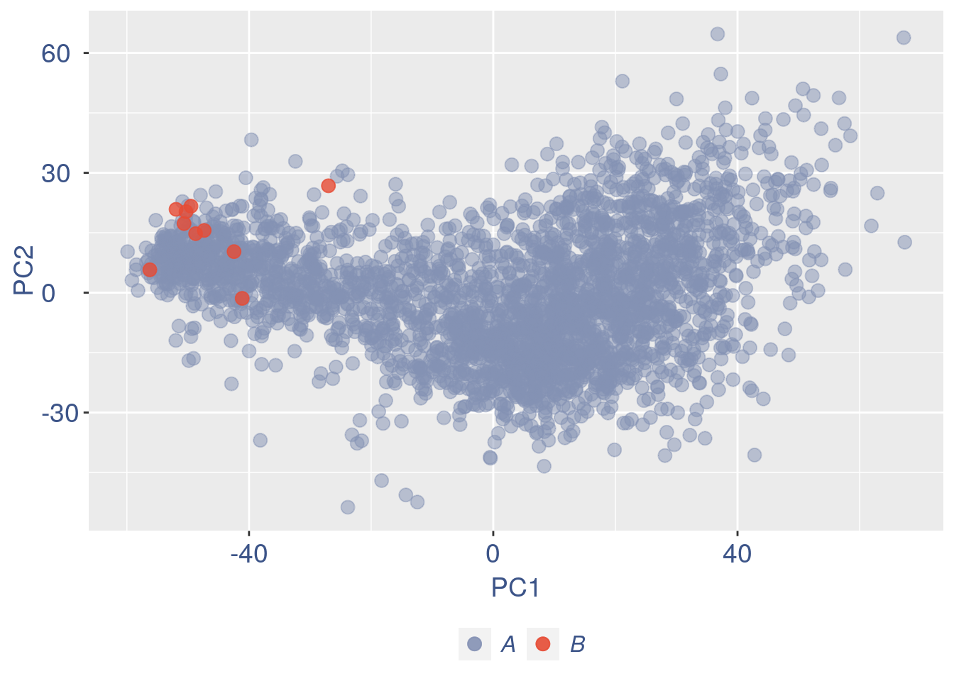
Just to check again, we plot the final efficiency coloured PCA.
nu_est = round(obj@nu, digits = 7)
plot.nu <- ggplot(ttm$pca_cells, aes(x = PC1,
    y = PC2, colour = log(nu_est)))
plot.nu = plot.nu + geom_point(size = 2,
    alpha = 0.8) + scale_color_gradient2(low = "#E64B35B2",
    mid = "#4DBBD5B2", high = "#3C5488B2",
    midpoint = log(mean(nu_est)), name = "ln(nu)") +
    ggtitle("Cells PCA coloured by cells efficiency: last") +
    my_theme + theme(plot.title = element_text(color = "#3C5488FF",
    size = 20), legend.title = element_text(color = "#3C5488FF",
    size = 14, face = "italic"), legend.text = element_text(color = "#3C5488FF",
    size = 13), legend.key.width = unit(2,
    "mm"), legend.position = "right")

pdf(paste(out_dir, "cleaning/", t, "_plots_PCA_efficiency_colored_FINAL.pdf",
    sep = ""))
plot.nu
dev.off()
#> png
#>   2

plot.nu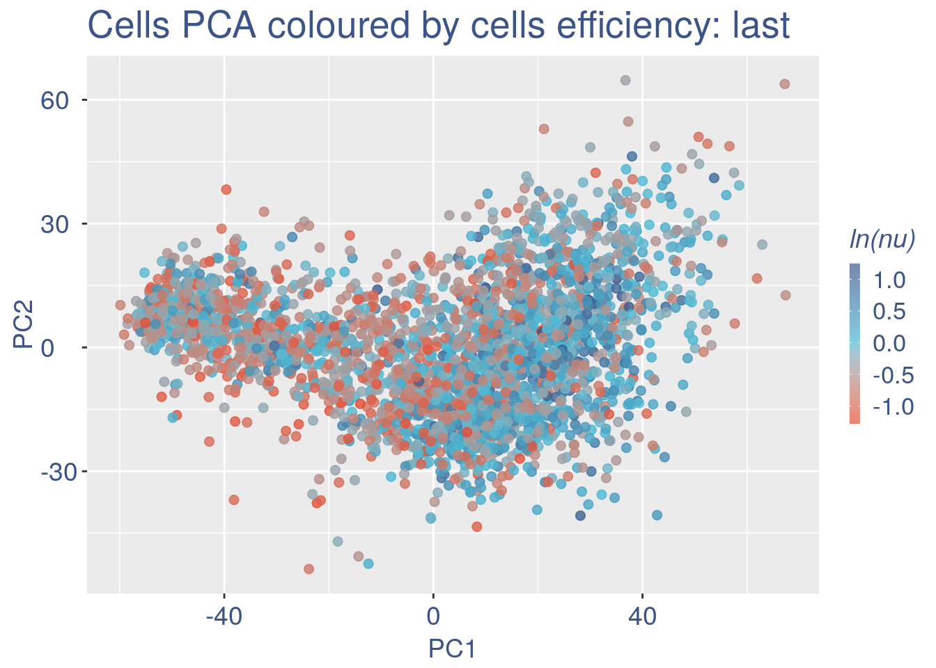
COTAN analysis: in this part all the contingency tables are computed and used to get the statistics (S) To storage efficiency of all the observed tables only the yes_yes is stored. Note that if will be necessary re-computing the yes-yes table, the yes-yes table should be cancelled before running cotan_analysis.
COEX evaluation and storing
saveRDS(obj, file = paste(out_dir, t, ".cotan.RDS",
    sep = ""))

obj = get.coex(obj)

# saving the structure
saveRDS(obj, file = paste(out_dir, t, ".cotan.RDS",
    sep = ""))
Automatic data elaboration (without cleaning)
3 Analysis of the elaborated data
In this case the test possible macroscopic differences between cleaned and not cleaned data.
The initial cell number was:
obj@meta
#>                         V1                 V2
#> 1                     GEO:          GSE107122
#> 2         scRNAseq method:            DropSeq
#> 3    starting n. of cells:               2955
#> 4        Condition sample: mouse cortex E15.5
#> 5 Threshold low UDE cells:               0.28
While the final number of cells was:
So were removed:
cells
3.1 GDI with cleaning
quant.p = get.GDI(obj)
#> [1] "function to generate GDI dataframe"
#> [1] "Using S"
#> [1] "function to generate S "

head(quant.p)
#>               sum.raw.norm      GDI exp.cells
#> 0610007N19Rik     6.029794 2.885667  7.663488
#> 0610007P14Rik     6.541578 1.567536 19.175749
#> 0610009B22Rik     6.522867 1.352988 18.698910
#> 0610009D07Rik     7.938454 1.378622 55.313351
#> 0610009E02Rik     3.924783 1.844979  1.498638
#> 0610009L18Rik     5.167619 1.273583  4.904632
In the third column of this data frame is reported the percentage of cells expressing the gene.
NPGs = c("Nes", "Vim", "Sox2", "Sox1", "Notch1",
    "Hes1", "Hes5", "Pax6")  #,'Hes3'
PNGs = c("Map2", "Tubb3", "Neurod1", "Nefm",
    "Nefl", "Dcx", "Tbr1")
hk = c("Calm1", "Cox6b1", "Ppia", "Rpl18",
    "Cox7c", "Erh", "H3f3a", "Taf1", "Taf2",
    "Gapdh", "Actb", "Golph3", "Mtmr12",
    "Zfr", "Sub1", "Tars", "Amacr")

text.size = 12

quant.p$highlight = with(quant.p, ifelse(rownames(quant.p) %in%
    NPGs, "NPGs", ifelse(rownames(quant.p) %in%
    hk, "Constitutive", ifelse(rownames(quant.p) %in%
    PNGs, "PNGs", "normal"))))

textdf <- quant.p[rownames(quant.p) %in%
    c(NPGs, hk, PNGs), ]
mycolours <- c(Constitutive = "#00A087FF",
    NPGs = "#E64B35FF", PNGs = "#F39B7FFF",
    normal = "#8491B4B2")
f1 = ggplot(subset(quant.p, highlight ==
    "normal"), aes(x = sum.raw.norm, y = GDI)) +
    geom_point(alpha = 0.1, color = "#8491B4B2",
        size = 2.5)
GDI_plot = f1 + geom_point(data = subset(quant.p,
    highlight != "normal"), aes(x = sum.raw.norm,
    y = GDI, colour = highlight), size = 2.5,
    alpha = 0.8) + geom_hline(yintercept = quantile(quant.p$GDI)[4],
    linetype = "dashed", color = "darkblue") +
    geom_hline(yintercept = quantile(quant.p$GDI)[3],
        linetype = "dashed", color = "darkblue") +
    geom_hline(yintercept = 1.5, linetype = "dotted",
        color = "red", size = 0.5) + scale_color_manual("Status",
    values = mycolours) + scale_fill_manual("Status",
    values = mycolours) + xlab("log normalized counts") +
    ylab("GDI") + geom_label_repel(data = textdf,
    aes(x = sum.raw.norm, y = GDI, label = rownames(textdf),
        fill = highlight), label.size = NA,
    alpha = 0.5, direction = "both", na.rm = TRUE,
    seed = 1234) + geom_label_repel(data = textdf,
    aes(x = sum.raw.norm, y = GDI, label = rownames(textdf)),
    label.size = NA, segment.color = "black",
    segment.size = 0.5, direction = "both",
    alpha = 0.8, na.rm = TRUE, fill = NA,
    seed = 1234) + theme(axis.text.x = element_text(size = text.size,
    angle = 0, hjust = 0.5, vjust = 0.5,
    face = "plain", colour = "#3C5488FF"),
    axis.text.y = element_text(size = text.size,
        angle = 0, hjust = 0, vjust = 0.5,
        face = "plain", colour = "#3C5488FF"),
    axis.title.x = element_text(size = text.size,
        angle = 0, hjust = 0.5, vjust = 0,
        face = "plain", colour = "#3C5488FF"),
    axis.title.y = element_text(size = text.size,
        angle = 90, hjust = 0.5, vjust = 0.5,
        face = "plain", colour = "#3C5488FF"),
    legend.title = element_blank(), legend.text = element_text(color = "#3C5488FF",
        face = "italic"), legend.position = "bottom")  # titl)
legend <- cowplot::get_legend(GDI_plot)
GDI_plot = GDI_plot + theme(legend.position = "none")
GDI_plot
3.2 GDI without cleaning
quant.p = get.GDI(obj2)
#> [1] "function to generate GDI dataframe"
#> [1] "Using S"
#> [1] "function to generate S "

head(quant.p)
#>               sum.raw.norm      GDI exp.cells
#> 0610007N19Rik     6.025327 2.881709  7.614213
#> 0610007P14Rik     6.537112 1.571894 19.052453
#> 0610009B22Rik     6.524282 1.355656 18.612521
#> 0610009D07Rik     7.935413 1.389342 54.991540
#> 0610009E02Rik     3.920299 1.845393  1.489002
#> 0610009L18Rik     5.163154 1.275495  4.873096
In the third column of this data frame is reported the percentage of cells expressing the gene.
NPGs = c("Nes", "Vim", "Sox2", "Sox1", "Notch1",
    "Hes1", "Hes5", "Pax6")  #,'Hes3'
PNGs = c("Map2", "Tubb3", "Neurod1", "Nefm",
    "Nefl", "Dcx", "Tbr1")
hk = c("Calm1", "Cox6b1", "Ppia", "Rpl18",
    "Cox7c", "Erh", "H3f3a", "Taf1", "Taf2",
    "Gapdh", "Actb", "Golph3", "Mtmr12",
    "Zfr", "Sub1", "Tars", "Amacr")

text.size = 12

quant.p$highlight = with(quant.p, ifelse(rownames(quant.p) %in%
    NPGs, "NPGs", ifelse(rownames(quant.p) %in%
    hk, "Constitutive", ifelse(rownames(quant.p) %in%
    PNGs, "PNGs", "normal"))))

textdf <- quant.p[rownames(quant.p) %in%
    c(NPGs, hk, PNGs), ]
mycolours <- c(Constitutive = "#00A087FF",
    NPGs = "#E64B35FF", PNGs = "#F39B7FFF",
    normal = "#8491B4B2")
f1 = ggplot(subset(quant.p, highlight ==
    "normal"), aes(x = sum.raw.norm, y = GDI)) +
    geom_point(alpha = 0.1, color = "#8491B4B2",
        size = 2.5)
GDI_plot = f1 + geom_point(data = subset(quant.p,
    highlight != "normal"), aes(x = sum.raw.norm,
    y = GDI, colour = highlight), size = 2.5,
    alpha = 0.8) + geom_hline(yintercept = quantile(quant.p$GDI)[4],
    linetype = "dashed", color = "darkblue") +
    geom_hline(yintercept = quantile(quant.p$GDI)[3],
        linetype = "dashed", color = "darkblue") +
    geom_hline(yintercept = 1.5, linetype = "dotted",
        color = "red", size = 0.5) + scale_color_manual("Status",
    values = mycolours) + scale_fill_manual("Status",
    values = mycolours) + xlab("log normalized counts") +
    ylab("GDI") + geom_label_repel(data = textdf,
    aes(x = sum.raw.norm, y = GDI, label = rownames(textdf),
        fill = highlight), label.size = NA,
    alpha = 0.5, direction = "both", na.rm = TRUE,
    seed = 1234) + geom_label_repel(data = textdf,
    aes(x = sum.raw.norm, y = GDI, label = rownames(textdf)),
    label.size = NA, segment.color = "black",
    segment.size = 0.5, direction = "both",
    alpha = 0.8, na.rm = TRUE, fill = NA,
    seed = 1234) + theme(axis.text.x = element_text(size = text.size,
    angle = 0, hjust = 0.5, vjust = 0.5,
    face = "plain", colour = "#3C5488FF"),
    axis.text.y = element_text(size = text.size,
        angle = 0, hjust = 0, vjust = 0.5,
        face = "plain", colour = "#3C5488FF"),
    axis.title.x = element_text(size = text.size,
        angle = 0, hjust = 0.5, vjust = 0,
        face = "plain", colour = "#3C5488FF"),
    axis.title.y = element_text(size = text.size,
        angle = 90, hjust = 0.5, vjust = 0.5,
        face = "plain", colour = "#3C5488FF"),
    legend.title = element_blank(), legend.text = element_text(color = "#3C5488FF",
        face = "italic"), legend.position = "bottom")  # titl)
legend <- cowplot::get_legend(GDI_plot)
GDI_plot = GDI_plot + theme(legend.position = "none")
GDI_plot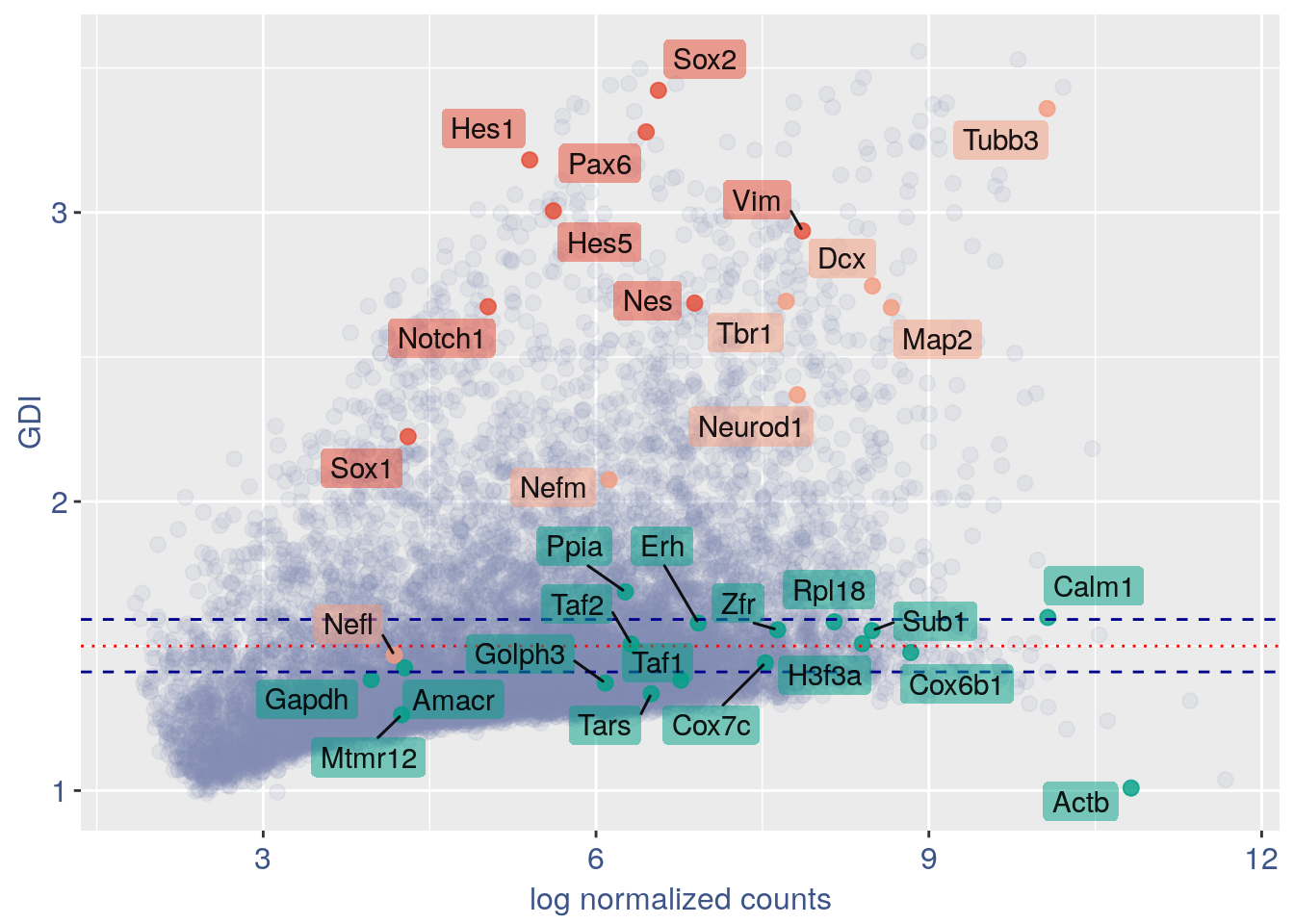
3.3 Heatmaps with cleaning
For the Gene Pair Analysis, we can plot an heatmap with the coex values between two genes sets. To do so we need to define, in a list, the different gene sets (list.genes). Then in the function parameter sets we can decide which sets need to be considered (in the example from 1 to 3). In the condition parameter we should insert an array with each file name prefix to be considered (in the example, the file names is “E15_cortex_clean”).
list.genes = list(Ref.col = PNGs, NPGs = NPGs,
    Const. = hk)

plot_heatmap(df_genes = list.genes, sets = c(1:3),
    conditions = "E15_cortex_clean", dir = "Data/")
#> [1] "plot heatmap"
#> [1] "Loading condition E15_cortex_clean"
#> [1] "Map2"    "Tubb3"   "Neurod1" "Nefm"    "Nefl"    "Dcx"     "Tbr1"
#> [1] "Get p-values on a set of genes on columns on a set of genes on rows"
#> [1] "Using function S"
#> [1] "function to generate S "
#> [1] "Ref.col"
#> [1] "NPGs"
#> [1] "Const."
#> [1] "min coex: -0.00726870963092396 max coex 0.00386426580215812"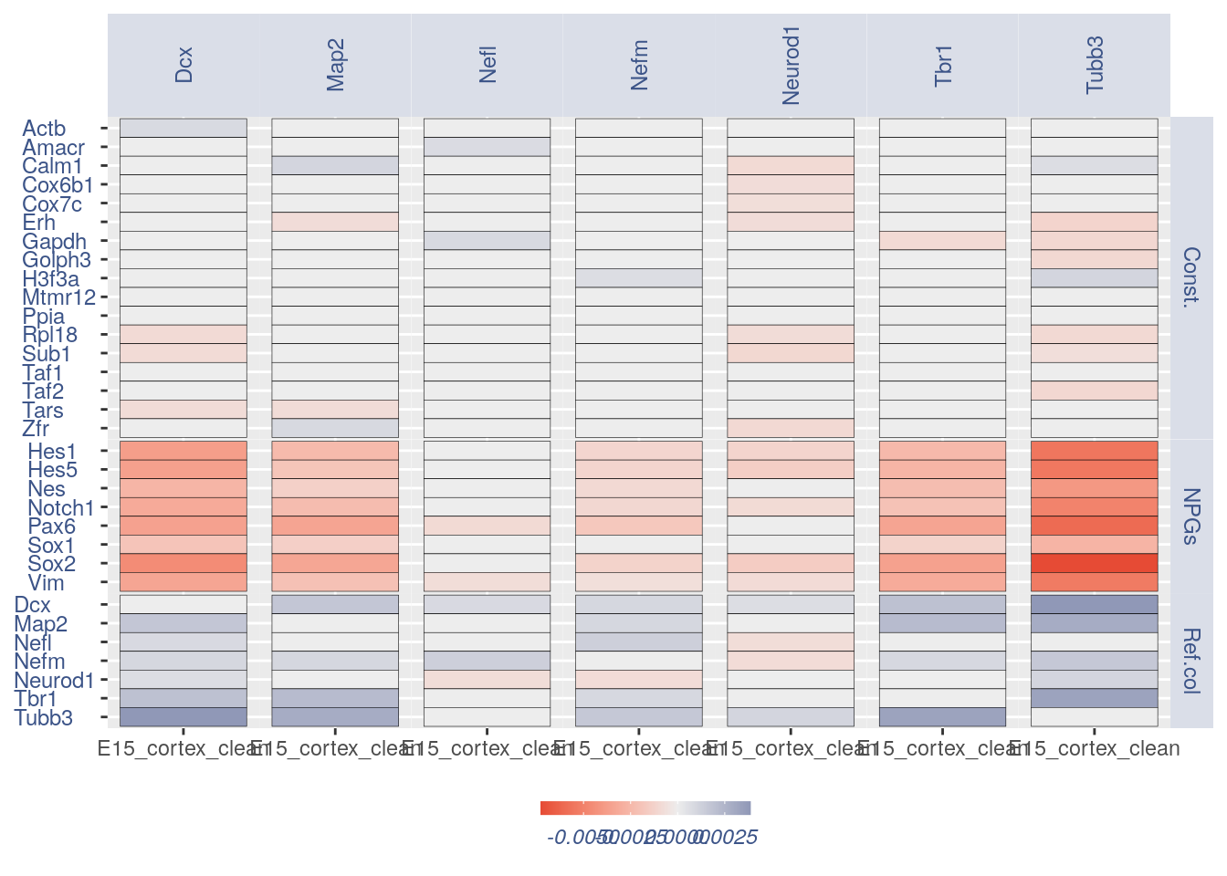
3.4 Heatmaps without cleaning
list.genes = list(Ref.col = PNGs, NPGs = NPGs,
    Const. = hk)

plot_heatmap(df_genes = list.genes, sets = c(1:3),
    conditions = "E15_cortex", dir = "Data/")
#> [1] "plot heatmap"
#> [1] "Loading condition E15_cortex"
#> [1] "Map2"    "Tubb3"   "Neurod1" "Nefm"    "Nefl"    "Dcx"     "Tbr1"
#> [1] "Get p-values on a set of genes on columns on a set of genes on rows"
#> [1] "Using function S"
#> [1] "function to generate S "
#> [1] "Ref.col"
#> [1] "NPGs"
#> [1] "Const."
#> [1] "min coex: -0.00724106834694776 max coex 0.00379181054369274"
print(sessionInfo())
#> R version 4.0.4 (2021-02-15)
#> Platform: x86_64-pc-linux-gnu (64-bit)
#> Running under: Ubuntu 18.04.5 LTS
#>
#> Matrix products: default
#> BLAS:   /usr/lib/x86_64-linux-gnu/openblas/libblas.so.3
#> LAPACK: /usr/lib/x86_64-linux-gnu/libopenblasp-r0.2.20.so
#>
#> locale:
#>  [1] LC_CTYPE=en_US.UTF-8       LC_NUMERIC=C
#>  [3] LC_TIME=en_US.UTF-8        LC_COLLATE=en_US.UTF-8
#>  [5] LC_MONETARY=en_US.UTF-8    LC_MESSAGES=en_US.UTF-8
#>  [7] LC_PAPER=en_US.UTF-8       LC_NAME=C
#>  [9] LC_ADDRESS=C               LC_TELEPHONE=C
#> [11] LC_MEASUREMENT=en_US.UTF-8 LC_IDENTIFICATION=C
#>
#> attached base packages:
#> [1] stats     graphics  grDevices utils     datasets  methods   base
#>
#> other attached packages:
#> [1] ggrepel_0.9.1     ggplot2_3.3.3     Matrix_1.3-2      data.table_1.14.0
#> [5] COTAN_0.1.0
#>
#> loaded via a namespace (and not attached):
#>  [1] sass_0.3.1           tidyr_1.1.2          jsonlite_1.7.2
#>  [4] R.utils_2.10.1       bslib_0.2.4          assertthat_0.2.1
#>  [7] highr_0.8            stats4_4.0.4         yaml_2.2.1
#> [10] pillar_1.5.1         lattice_0.20-41      glue_1.4.2
#> [13] reticulate_1.18      digest_0.6.27        RColorBrewer_1.1-2
#> [16] colorspace_2.0-0     cowplot_1.1.1        htmltools_0.5.1.1
#> [19] R.oo_1.24.0          pkgconfig_2.0.3      GetoptLong_1.0.5
#> [22] purrr_0.3.4          scales_1.1.1         tibble_3.1.0
#> [25] generics_0.1.0       farver_2.1.0         IRanges_2.24.1
#> [28] ellipsis_0.3.1       withr_2.4.1          BiocGenerics_0.36.0
#> [31] magrittr_2.0.1       crayon_1.4.0         evaluate_0.14
#> [34] R.methodsS3_1.8.1    fansi_0.4.2          Cairo_1.5-12.2
#> [37] tools_4.0.4          GlobalOptions_0.1.2  formatR_1.8
#> [40] lifecycle_1.0.0      matrixStats_0.58.0   ComplexHeatmap_2.6.2
#> [43] basilisk.utils_1.2.2 stringr_1.4.0        S4Vectors_0.28.1
#> [46] munsell_0.5.0        cluster_2.1.1        compiler_4.0.4
#> [49] jquerylib_0.1.3      rlang_0.4.10         grid_4.0.4
#> [52] rjson_0.2.20         rappdirs_0.3.3       circlize_0.4.12
#> [55] labeling_0.4.2       rmarkdown_2.7        basilisk_1.2.1
#> [58] gtable_0.3.0         DBI_1.1.1            R6_2.5.0
#> [61] knitr_1.31           dplyr_1.0.4          utf8_1.2.1
#> [64] clue_0.3-58          filelock_1.0.2       shape_1.4.5
#> [67] stringi_1.5.3        parallel_4.0.4       Rcpp_1.0.6
#> [70] vctrs_0.3.6          png_0.1-7            tidyselect_1.1.0
#> [73] xfun_0.22