E13.5 cortex
library(COTAN)
library(data.table)
library(Matrix)
library(ggrepel)
#> Loading required package: ggplot2
# library(latex2exp)
mycolours <- c(A = "#8491B4B2", B = "#E64B35FF")
my_theme = theme(axis.text.x = element_text(size = 14,
angle = 0, hjust = 0.5, vjust = 0.5,
face = "plain", colour = "#3C5488FF"),
axis.text.y = element_text(size = 14,
angle = 0, hjust = 0, vjust = 0.5,
face = "plain", colour = "#3C5488FF"),
axis.title.x = element_text(size = 14,
angle = 0, hjust = 0.5, vjust = 0,
face = "plain", colour = "#3C5488FF"),
axis.title.y = element_text(size = 14,
angle = 90, hjust = 0.5, vjust = 0.5,
face = "plain", colour = "#3C5488FF"))data = as.data.frame(fread(paste(data_dir,
"GSM2861511_E135_Only_Cortical_Cells_DGE.txt.gz",
sep = "/")))
data = as.data.frame(data)
rownames(data) = data$V1
data = data[, 2:ncol(data)]
data[1:10, 1:10]
#> GTAGCAATTTCT TACTAGATGCTA TATCAGCAGATT TACAGGCCCGTC TGATATACACTT
#> 0610005C13Rik 0 0 0 0 0
#> 0610007N19Rik 0 0 2 0 0
#> 0610007P14Rik 0 0 1 1 0
#> 0610009B22Rik 0 1 0 0 1
#> 0610009D07Rik 0 2 1 0 2
#> 0610009E02Rik 0 0 0 0 0
#> 0610009L18Rik 1 0 0 0 0
#> 0610009O20Rik 0 0 0 0 0
#> 0610010F05Rik 1 4 2 4 1
#> 0610010K14Rik 0 0 0 0 0
#> ATTTCGCGTGAA GGTTTGTCCTTT AACGTCACATCC CCTATCCTTTGC AAATTCGTCGGT
#> 0610005C13Rik 0 0 0 0 0
#> 0610007N19Rik 0 0 0 0 0
#> 0610007P14Rik 1 0 1 0 0
#> 0610009B22Rik 0 0 0 0 0
#> 0610009D07Rik 0 4 2 0 2
#> 0610009E02Rik 0 0 0 0 0
#> 0610009L18Rik 0 0 0 0 0
#> 0610009O20Rik 0 0 0 0 0
#> 0610010F05Rik 2 0 4 3 1
#> 0610010K14Rik 0 0 0 0 0Define a directory where the ouput will be stored.
1 Analytical pipeline
Initialize the COTAN object with the row count table and the metadata for the experiment.
obj = new("scCOTAN", raw = data)
obj = initRaw(obj, GEO = "GSM2861511", sc.method = "DropSeq",
    cond = "mouse cortex E13.5")
#> [1] "Initializing S4 object"
Now we can start the cleaning. Analysis requires and starts from a matrix of raw UMI counts after removing possible cell doublets or multiplets and low quality or dying cells (with too high mtRNA percentage, easily done with Seurat or other tools).
If we do not want to consider the mitochondrial genes we can remove them before starting the analysis.
genes_to_rem = rownames(obj@raw[grep("^mt",
    rownames(obj@raw)), ])  #genes to remove : mithocondrial
obj@raw = obj@raw[!rownames(obj@raw) %in%
    genes_to_rem, ]
cells_to_rem = colnames(obj@raw[which(colSums(obj@raw) ==
    0)])
obj@raw = obj@raw[, !colnames(obj@raw) %in%
    cells_to_rem]
We want also to define a prefix to identify the sample.
t = "E13_cortex_clean"

print(paste("Condition ", t, sep = ""))
#> [1] "Condition E13_cortex_clean"
#--------------------------------------
n_cells = length(colnames(obj@raw))
print(paste("n cells", n_cells, sep = " "))
#> [1] "n cells 1137"

n_it = 1

# obj@raw = obj@raw[rownames(cells),
# colnames(cells)]
2 Data cleaning
First we create the directory to store all information regardin the data cleaning.
if (!file.exists(out_dir)) {
    dir.create(file.path(out_dir))
}

if (!file.exists(paste(out_dir, "cleaning",
    sep = ""))) {
    dir.create(file.path(out_dir, "cleaning"))
}
ttm = clean(obj)
#> [1] "Start estimation mu with linear method"
#> [1] 12725 1137
#> rowname TCTATACAACGA
#> 5286 Hbb-bs 324.117944
#> 5283 Hba-a1 236.415441
#> 5287 Hbb-bt 129.647177
#> 698 Actb 27.963117
#> 11282 Tmsb4x 20.336812
#> 2258 Cfl1 10.168406
#> 5004 Gnas 10.168406
#> 7757 Pabpc1 10.168406
#> 1807 Calm1 8.897355
#> 5611 Igf2 7.626305
#> 6418 Malat1 7.626305
#> 8043 Pfn1 7.626305
#> 9800 Serpinh1 7.626305
#> 10048 Slc25a5 7.626305
#> 10063 Slc2a1 7.626305
obj = ttm$object
ttm$pca.cell.2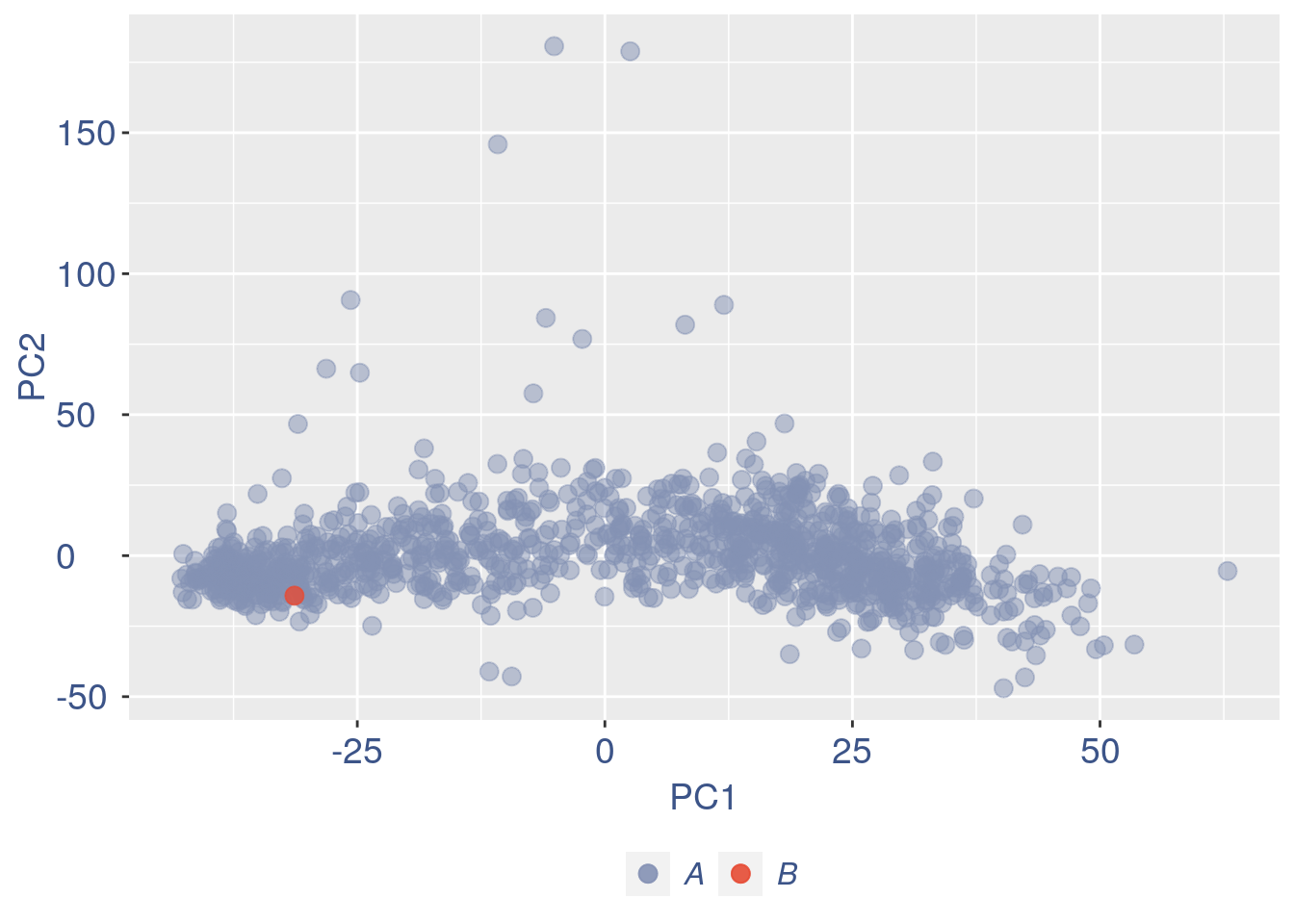
Run this when B cells need to be removed.
pdf(paste(out_dir, "cleaning/", t, "_", n_it,
    "_plots_before_cells_exlusion.pdf", sep = ""))
ttm$pca.cell.2
ggplot(ttm$D, aes(x = n, y = means)) + geom_point() +
    geom_text_repel(data = subset(ttm$D,
        n > (max(ttm$D$n) - 15)), aes(n,
        means, label = rownames(ttm$D[ttm$D$n >
            (max(ttm$D$n) - 15), ])), nudge_y = 0.05,
        nudge_x = 0.05, direction = "x",
        angle = 90, vjust = 0, segment.size = 0.2) +
    ggtitle("B cell group genes mean expression") +
    my_theme + theme(plot.title = element_text(color = "#3C5488FF",
    size = 20, face = "italic", vjust = -5,
    hjust = 0.02))
dev.off()
#> png
#>   2

if (length(ttm$cl1) < length(ttm$cl2)) {
    to_rem = ttm$cl1
} else {
    to_rem = ttm$cl2
}
n_it = n_it + 1
obj@raw = obj@raw[, !colnames(obj@raw) %in%
    to_rem]
# obj@raw = obj@raw[rownames(obj@raw)
# %in% rownames(cells),colnames(obj@raw)
# %in% colnames(cells)]
gc()
#>            used  (Mb) gc trigger   (Mb)  max used  (Mb)
#> Ncells  3734347 199.5    6027567  322.0   6027567 322.0
#> Vcells 98496308 751.5  144889565 1105.5 120674318 920.7

ttm = clean(obj)
#> [1] "Start estimation mu with linear method"
#> [1] 12714  1136
#>       rowname AAATCCCTAAAG
#> 6410   Malat1     78.03508
#> 7749   Pabpc1     48.77192
#> 3802  Fam168a     39.01754
#> 11592   Ttyh1     39.01754
#> 12214  Zbtb41     39.01754
#> 2720   Ctnna1     29.26315
#> 10789   Taf1d     29.26315
#> 1119   Arglu1     19.50877
#> 1247    Ash1l     19.50877
#> 1717   Bzrap1     19.50877
#> 1789   Cacng4     19.50877
#> 2581   Cox7a2     19.50877
#> 4266     Gas5     19.50877
#> 5075    Gpm6b     19.50877
#> 5606  Igf2bp2     19.50877
# ttm = clean.sqrt(obj, cells)
obj = ttm$object

ttm$pca.cell.2
#> png
#>   2
#>             used  (Mb) gc trigger   (Mb)  max used   (Mb)
#> Ncells   3734576 199.5    6027567  322.0   6027567  322.0
#> Vcells 100857214 769.5  250660367 1912.4 250659663 1912.4
#> [1] "Start estimation mu with linear method"
#> [1] 12714  1135
#>             rowname TTACATTGACCA GAGTTCCTCTTA TTTAAAATACAC
#> 6410         Malat1   164.870988   212.781146    203.06089
#> 6627           Meg3     0.000000     3.940392     43.07352
#> 7334           Nfib     0.000000     0.000000     43.07352
#> 10898          Tcf4    36.065529     0.000000      6.15336
#> 9038          Rbm25     0.000000    11.821175     24.61344
#> 12111          Xist    36.065529     0.000000      0.00000
#> 248   2810055G20Rik    15.456655    15.761566      0.00000
#> 3507          Eif5b    10.304437    19.701958      0.00000
#> 8759          Ptprs    10.304437     0.000000     18.46008
#> 10519         Srrm1    20.608874     7.880783      0.00000
#> 1382           Atrx    10.304437    11.821175      6.15336
#> 11281          Tmx4     0.000000     0.000000     24.61344
#> 5132          Gria2     5.152218     0.000000     18.46008
#> 10522         Srrm4    10.304437     0.000000     12.30672
#> 6038          Kmt2a     0.000000     3.940392     18.46008
Run this only in the last iteration, instead the previous code, when B cells group has not to be removed.
pdf(paste(out_dir, "cleaning/", t, "_", n_it,
    "_plots_before_cells_exlusion.pdf", sep = ""))
ttm$pca.cell.2
ggplot(ttm$D, aes(x = n, y = means)) + geom_point() +
    geom_text_repel(data = subset(ttm$D,
        n > (max(ttm$D$n) - 15)), aes(n,
        means, label = rownames(ttm$D[ttm$D$n >
            (max(ttm$D$n) - 15), ])), nudge_y = 0.05,
        nudge_x = 0.05, direction = "x",
        angle = 90, vjust = 0, segment.size = 0.2) +
    ggtitle(label = "B cell group genes mean expression",
        subtitle = " - B group NOT removed -") +
    my_theme + theme(plot.title = element_text(color = "#3C5488FF",
    size = 20, face = "italic", vjust = -10,
    hjust = 0.02), plot.subtitle = element_text(color = "darkred",
    vjust = -15, hjust = 0.01))

dev.off()
#> png
#>   2
To color the pca based on nu_j (so the cells’ efficiency).
nu_est = round(obj@nu, digits = 7)

plot.nu <- ggplot(ttm$pca_cells, aes(x = PC1,
    y = PC2, colour = log(nu_est)))

plot.nu = plot.nu + geom_point(size = 1,
    alpha = 0.8) + scale_color_gradient2(low = "#E64B35B2",
    mid = "#4DBBD5B2", high = "#3C5488B2",
    midpoint = log(mean(nu_est)), name = "ln (nu)") +
    ggtitle("Cells PCA coloured by cells efficiency") +
    my_theme + theme(plot.title = element_text(color = "#3C5488FF",
    size = 20), legend.title = element_text(color = "#3C5488FF",
    size = 14, face = "italic"), legend.text = element_text(color = "#3C5488FF",
    size = 13), legend.key.width = unit(2,
    "mm"), legend.position = "right")

pdf(paste(out_dir, "cleaning/", t, "_plots_PCA_efficiency_colored.pdf",
    sep = ""))
plot.nu
dev.off()
#> png
#>   2

plot.nu
The next part is use to remove the cells with efficiency too low.
nu_df = data.frame(nu = sort(obj@nu), n = c(1:length(obj@nu)))

ggplot(nu_df, aes(x = n, y = nu)) + geom_point(colour = "#8491B4B2",
    size = 1) + my_theme  #+ ylim(0,1) + xlim(0,70)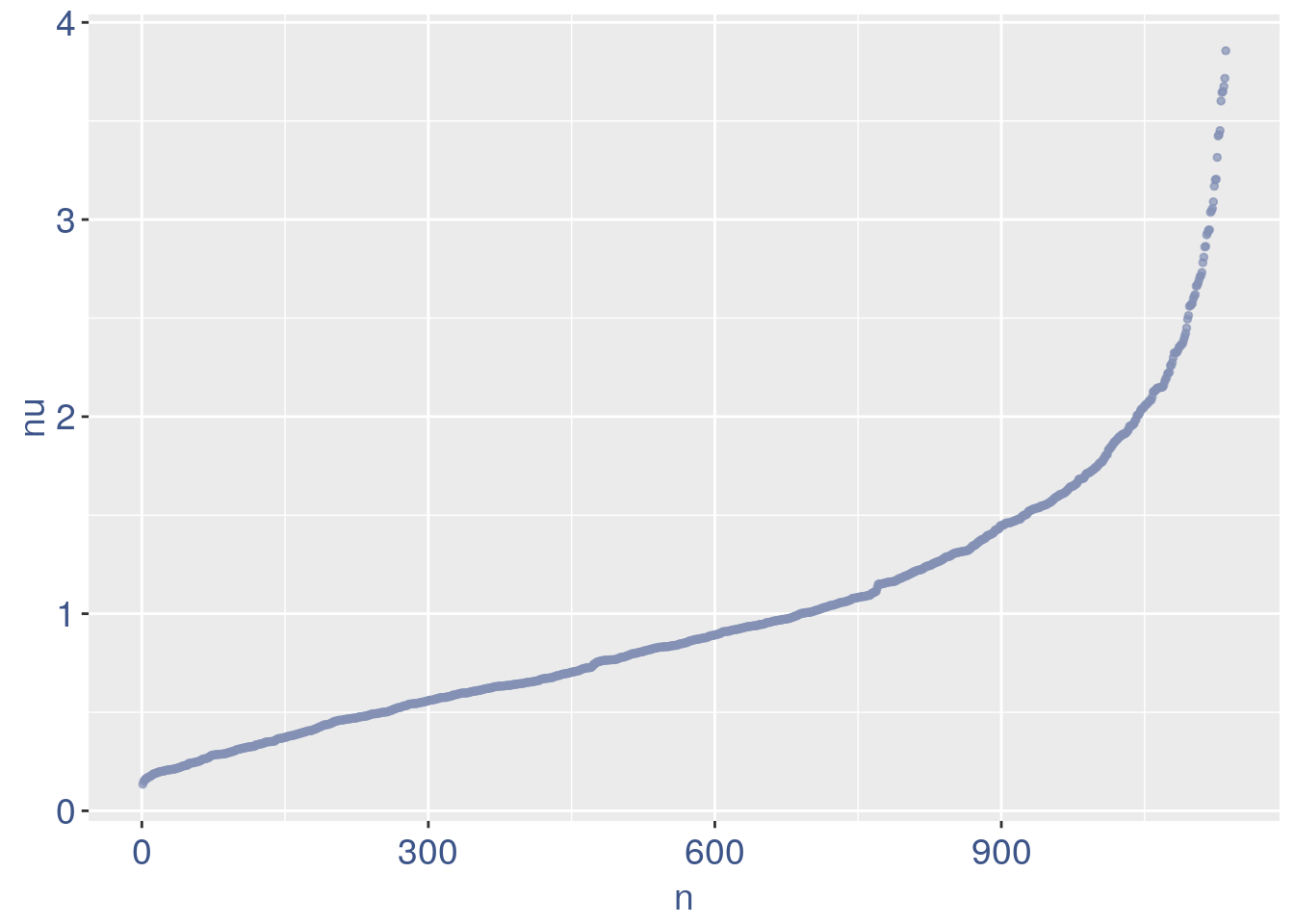
We can zoom on the smalest values and, if we detect a clear elbow, we can decide to remove the cells.
yset = 0.18  #threshold to remove low UDE cells
plot.ude <- ggplot(nu_df, aes(x = n, y = nu)) +
    geom_point(colour = "#8491B4B2", size = 1) +
    my_theme + ylim(0, 0.5) + xlim(0, 200) +
    geom_hline(yintercept = yset, linetype = "dashed",
        color = "darkred") + annotate(geom = "text",
    x = 500, y = 0.5, label = paste("to remove cells with nu < ",
        yset, sep = " "), color = "darkred",
    size = 4.5)


pdf(paste(out_dir, "cleaning/", t, "_plots_efficiency.pdf",
    sep = ""))
plot.ude
dev.off()
#> png
#>   2

plot.ude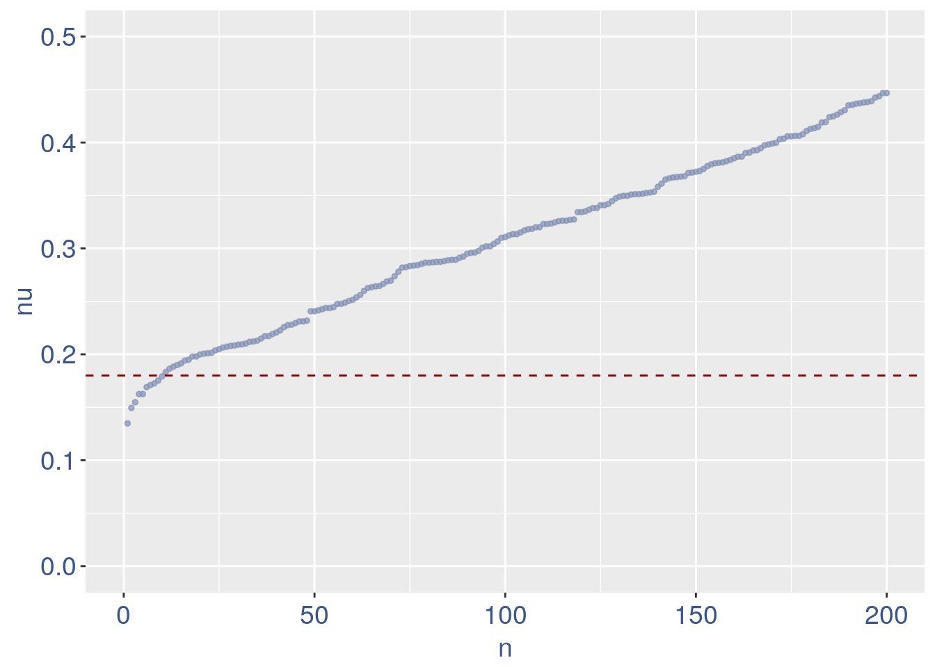
We also save the defined treshold in the metadata and re run the estimation
obj@meta[(nrow(obj@meta) + 1), 1:2] = c("Threshold low UDE cells:",
    yset)

to_rem = rownames(nu_df[which(nu_df$nu <
    yset), ])

obj@raw = obj@raw[, !colnames(obj@raw) %in%
    to_rem]
Repeat the estimation after the cells are removed
ttm = clean(obj)
#> [1] "Start estimation mu with linear method"
#> [1] 12708  1125
#>             rowname TTACATTGACCA GAGTTCCTCTTA
#> 6405         Malat1    166.09642   214.362683
#> 10892          Tcf4     36.33359     0.000000
#> 12105          Xist     36.33359     0.000000
#> 248   2810055G20Rik     15.57154    15.878717
#> 3504          Eif5b     10.38103    19.848397
#> 10513         Srrm1     20.76205     7.939359
#> 1380           Atrx     10.38103    11.909038
#> 11011         Tial1     10.38103    11.909038
#> 3509         Elavl2     20.76205     0.000000
#> 7414           Nnat     20.76205     0.000000
#> 10203          Smc4     20.76205     0.000000
#> 10369        Sorbs2     20.76205     0.000000
#> 1161         Arid4b      0.00000    19.848397
#> 8594        Prpf38b     15.57154     3.969679
#> 3248         Dpysl3     10.38103     7.939359
obj = ttm$object
ttm$pca.cell.2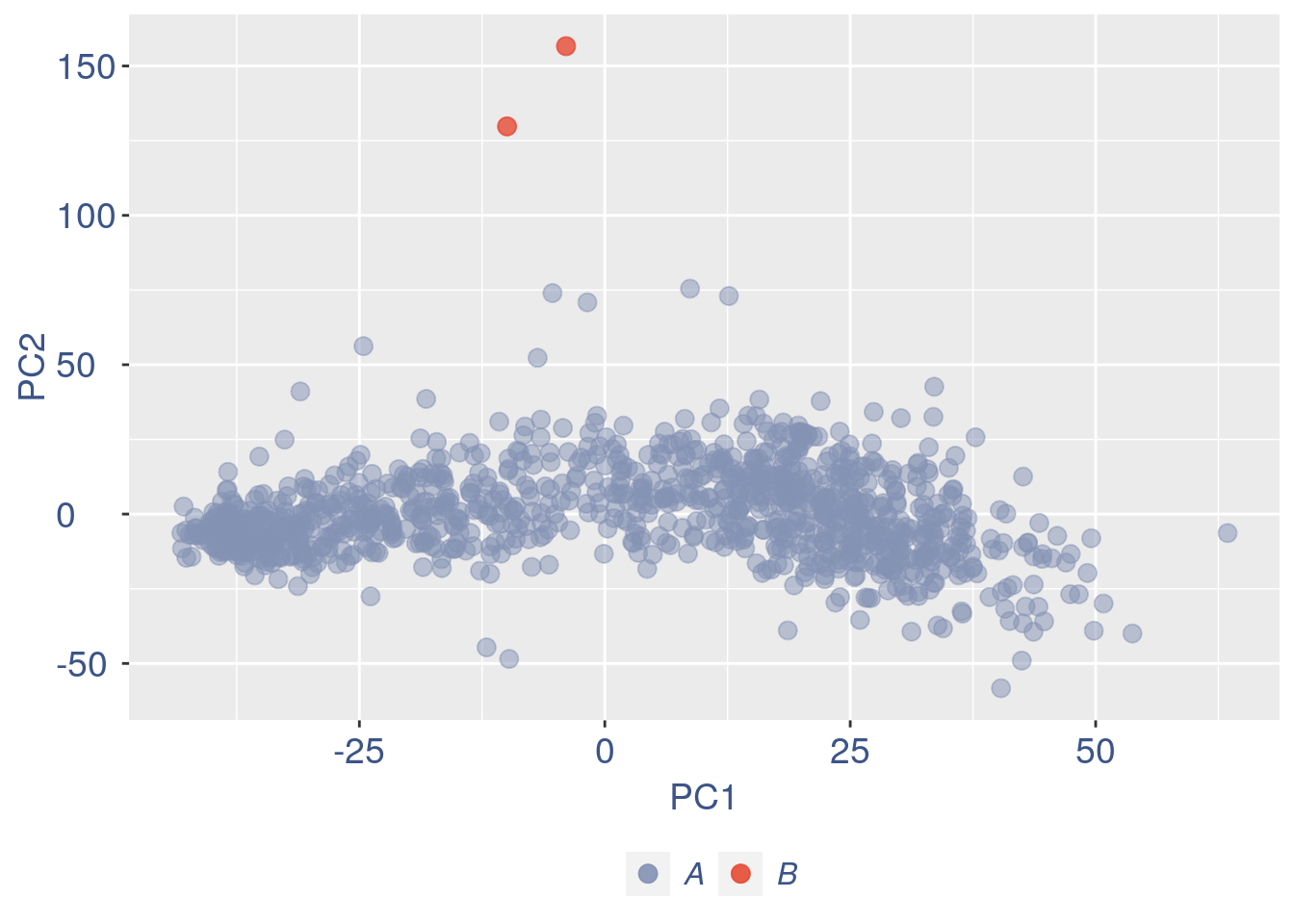
Just to check again, we plot the final efficiency colored PCA
nu_est = round(obj@nu, digits = 7)
plot.nu <- ggplot(ttm$pca_cells, aes(x = PC1,
    y = PC2, colour = log(nu_est)))
plot.nu = plot.nu + geom_point(size = 2,
    alpha = 0.8) + scale_color_gradient2(low = "#E64B35B2",
    mid = "#4DBBD5B2", high = "#3C5488B2",
    midpoint = log(mean(nu_est)), name = "ln(nu)") +
    ggtitle("Cells PCA coloured by cells efficiency: last") +
    my_theme + theme(plot.title = element_text(color = "#3C5488FF",
    size = 20), legend.title = element_text(color = "#3C5488FF",
    size = 14, face = "italic"), legend.text = element_text(color = "#3C5488FF",
    size = 13), legend.key.width = unit(2,
    "mm"), legend.position = "right")

pdf(paste(out_dir, "cleaning/", t, "_plots_PCA_efficiency_colored_FINAL.pdf",
    sep = ""))
plot.nu
dev.off()
#> png
#>   2

plot.nu
COTAN analysis: in this part all the contingency tables are computed and used to get the statistics (S) To storage efficiency of all the observed tables only the yes_yes is stored. Note that if will be necessary re-computing the yes-yes table, the yes-yes table should be cancelled before running cotan_analysis.
COEX evaluation and storing
saveRDS(obj, file = paste(out_dir, t, ".cotan.RDS",
    sep = ""))

obj = get.coex(obj)

# saving the structure
saveRDS(obj, file = paste(out_dir, t, ".cotan.RDS",
    sep = ""))
Automatic data elaboration (without cleaning)
obj2 = automatic.COTAN.object.creation(df = data,
    GEO = "GSM2861510", sc.method = "Drop-seq",
    cond = "E13_cortex", out_dir = "Data/")
#> [1] "Initializing S4 object"
#> [1] "Condition E13_cortex"
#> [1] "n cells 1137"
#> [1] "Start estimation mu with linear method"
#> [1] 12725  1137
#>        rowname TCTATACAACGA
#> 5286    Hbb-bs   324.117944
#> 5283    Hba-a1   236.415441
#> 5287    Hbb-bt   129.647177
#> 698       Actb    27.963117
#> 11282   Tmsb4x    20.336812
#> 2258      Cfl1    10.168406
#> 5004      Gnas    10.168406
#> 7757    Pabpc1    10.168406
#> 1807     Calm1     8.897355
#> 5611      Igf2     7.626305
#> 6418    Malat1     7.626305
#> 8043      Pfn1     7.626305
#> 9800  Serpinh1     7.626305
#> 10048  Slc25a5     7.626305
#> 10063   Slc2a1     7.626305
#> [1] "Cotan analysis function started"
#> [1] "cotan analysis"
#> [1] "mu estimator creation"
#> [1] "save effective constitutive genes"
#> [1] "start a minimization"
#> [1] "Next gene: Calml3 number 1810"
#> [1] "Next gene: Fam181a number 3820"
#> [1] "Next gene: Kank2 number 5830"
#> [1] "Next gene: Parva number 7840"
#> [1] "Next gene: Sfxn1 number 9850"
#> [1] "Next gene: Usp31 number 11860"
#> [1] "Final trance!"
#> [1] "a min: -0.0412673950195312 | a max 748.25 | negative a %: 10.9705304518664"
#> [1] "Only analysis time 0.786702223618825"
#> [1] "Cotan coex estimation started"
#> [1] "coex dataframe creation"
#> [1] "Generating contingency tables for observed data"
#> [1] "creation of observed yes/yes contingency table"
#> [1] "mu estimator creation"
#> [1] "expected contingency tables creation"
#> [1] "The distance between estimated n of zeros and observed number of zero is 0.0602744425111541 over 12725"
#> [1] "Done"
#> [1] "coex estimation"
#> [1] "Diagonal coex values substituted with 0"
#> [1] "Total time 2.61206785837809"
#> [1] "Only coex time 1.70640178918838"
#> [1] "Saving elaborated data locally at Data/E13_cortex.cotan.RDS"
3 Analysis of the elaborated data
In this case the test possible macroscopic differences between cleaned and not cleaned data.
The initial cell number was:
obj = readRDS(paste(out_dir, t, ".cotan.RDS",
    sep = ""))
obj@meta
#>                         V1                 V2
#> 1                     GEO:         GSM2861511
#> 2         scRNAseq method:            DropSeq
#> 3    starting n. of cells:               1137
#> 4        Condition sample: mouse cortex E13.5
#> 5 Threshold low UDE cells:               0.18
While the final number of cells was:
So were removed:
cells
3.1 GDI with cleaning
quant.p = get.GDI(obj)
#> [1] "function to generate GDI dataframe"
#> [1] "Using S"
#> [1] "function to generate S "

head(quant.p)
#>               sum.raw.norm      GDI exp.cells
#> 0610007N19Rik     5.166481 2.188999 10.133333
#> 0610007P14Rik     5.362836 1.677978 16.266667
#> 0610009B22Rik     5.375005 1.298590 15.022222
#> 0610009D07Rik     6.813781 1.414547 46.044444
#> 0610009E02Rik     3.686037 1.789690  3.111111
#> 0610009L18Rik     3.269327 1.231394  2.400000
In the third column of this data frame is reported the percentage of cells expressing the gene.
NPGs = c("Nes", "Vim", "Sox2", "Sox1", "Notch1",
    "Hes1", "Hes5", "Pax6")  #,'Hes3'
PNGs = c("Map2", "Tubb3", "Neurod1", "Nefm",
    "Nefl", "Dcx", "Tbr1")
hk = c("Calm1", "Cox6b1", "Ppia", "Rpl18",
    "Cox7c", "Erh", "H3f3a", "Taf1", "Taf2",
    "Gapdh", "Actb", "Golph3", "Mtmr12",
    "Zfr", "Sub1", "Tars", "Amacr")

text.size = 12

quant.p$highlight = with(quant.p, ifelse(rownames(quant.p) %in%
    NPGs, "NPGs", ifelse(rownames(quant.p) %in%
    hk, "Constitutive", ifelse(rownames(quant.p) %in%
    PNGs, "PNGs", "normal"))))

textdf <- quant.p[rownames(quant.p) %in%
    c(NPGs, hk, PNGs), ]
mycolours <- c(Constitutive = "#00A087FF",
    NPGs = "#E64B35FF", PNGs = "#F39B7FFF",
    normal = "#8491B4B2")
f1 = ggplot(subset(quant.p, highlight ==
    "normal"), aes(x = sum.raw.norm, y = GDI)) +
    geom_point(alpha = 0.1, color = "#8491B4B2",
        size = 2.5)
GDI_plot = f1 + geom_point(data = subset(quant.p,
    highlight != "normal"), aes(x = sum.raw.norm,
    y = GDI, colour = highlight), size = 2.5,
    alpha = 0.8) + geom_hline(yintercept = quantile(quant.p$GDI)[4],
    linetype = "dashed", color = "darkblue") +
    geom_hline(yintercept = quantile(quant.p$GDI)[3],
        linetype = "dashed", color = "darkblue") +
    geom_hline(yintercept = 1.5, linetype = "dotted",
        color = "red", size = 0.5) + scale_color_manual("Status",
    values = mycolours) + scale_fill_manual("Status",
    values = mycolours) + xlab("log normalized counts") +
    ylab("GDI") + geom_label_repel(data = textdf,
    aes(x = sum.raw.norm, y = GDI, label = rownames(textdf),
        fill = highlight), label.size = NA,
    alpha = 0.5, direction = "both", na.rm = TRUE,
    seed = 1234) + geom_label_repel(data = textdf,
    aes(x = sum.raw.norm, y = GDI, label = rownames(textdf)),
    label.size = NA, segment.color = "black",
    segment.size = 0.5, direction = "both",
    alpha = 0.8, na.rm = TRUE, fill = NA,
    seed = 1234) + theme(axis.text.x = element_text(size = text.size,
    angle = 0, hjust = 0.5, vjust = 0.5,
    face = "plain", colour = "#3C5488FF"),
    axis.text.y = element_text(size = text.size,
        angle = 0, hjust = 0, vjust = 0.5,
        face = "plain", colour = "#3C5488FF"),
    axis.title.x = element_text(size = text.size,
        angle = 0, hjust = 0.5, vjust = 0,
        face = "plain", colour = "#3C5488FF"),
    axis.title.y = element_text(size = text.size,
        angle = 90, hjust = 0.5, vjust = 0.5,
        face = "plain", colour = "#3C5488FF"),
    legend.title = element_blank(), legend.text = element_text(color = "#3C5488FF",
        face = "italic"), legend.position = "bottom")  # titl)
legend <- cowplot::get_legend(GDI_plot)
GDI_plot = GDI_plot + theme(legend.position = "none")
GDI_plot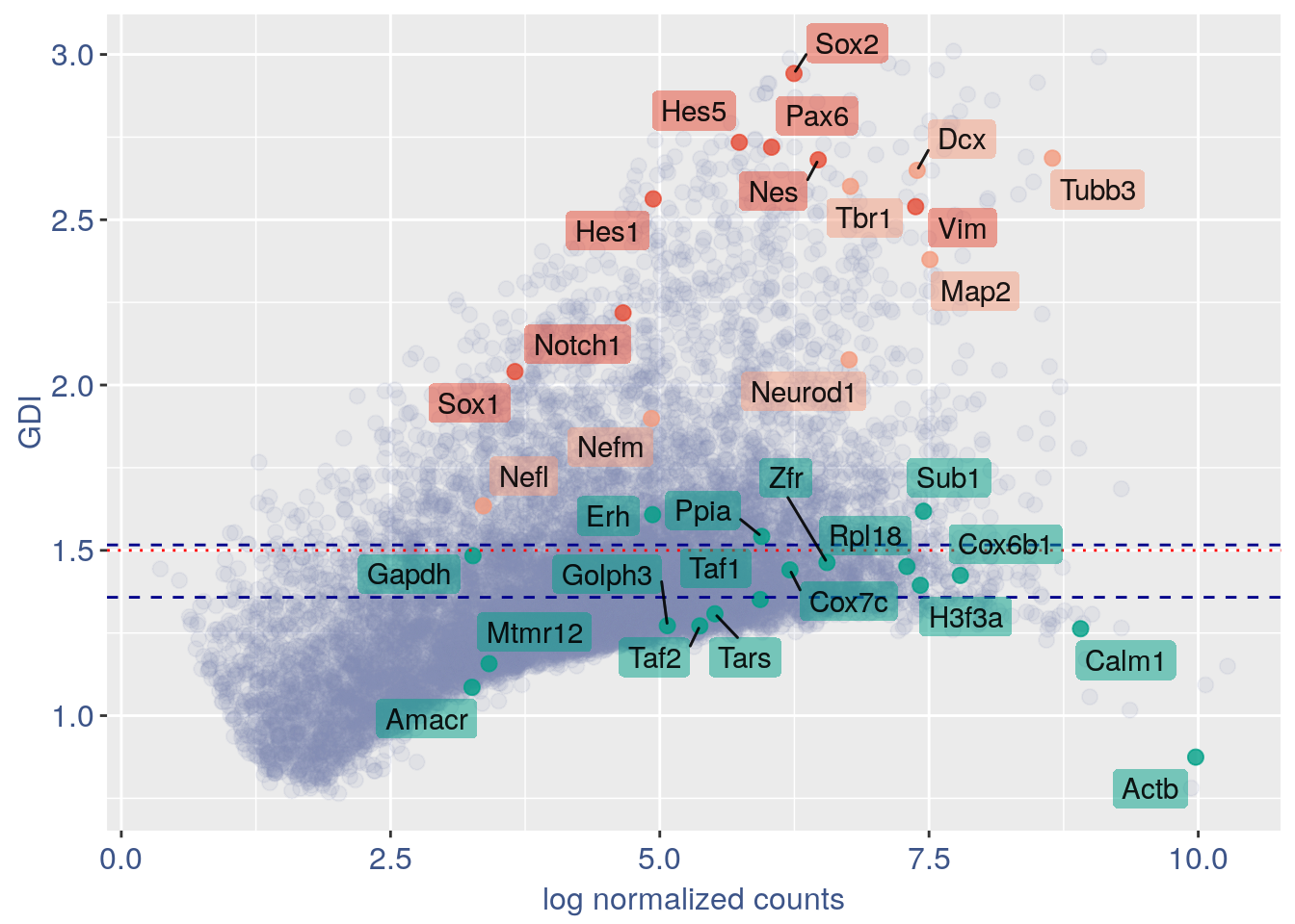
3.2 GDI without cleaning
quant.p = get.GDI(obj2)
#> [1] "function to generate GDI dataframe"
#> [1] "Using S"
#> [1] "function to generate S "

head(quant.p)
#>               sum.raw.norm      GDI exp.cells
#> 0610007N19Rik     5.158090 2.187929 10.026385
#> 0610007P14Rik     5.354445 1.686117 16.094987
#> 0610009B22Rik     5.366608 1.301230 14.863676
#> 0610009D07Rik     6.805391 1.410419 45.558487
#> 0610009E02Rik     3.677533 1.789017  3.078276
#> 0610009L18Rik     3.260923 1.231797  2.374670
In the third column of this data frame is reported the percentage of cells expressing the gene.
NPGs = c("Nes", "Vim", "Sox2", "Sox1", "Notch1",
    "Hes1", "Hes5", "Pax6")  #,'Hes3'
PNGs = c("Map2", "Tubb3", "Neurod1", "Nefm",
    "Nefl", "Dcx", "Tbr1")
hk = c("Calm1", "Cox6b1", "Ppia", "Rpl18",
    "Cox7c", "Erh", "H3f3a", "Taf1", "Taf2",
    "Gapdh", "Actb", "Golph3", "Mtmr12",
    "Zfr", "Sub1", "Tars", "Amacr")

text.size = 12

quant.p$highlight = with(quant.p, ifelse(rownames(quant.p) %in%
    NPGs, "NPGs", ifelse(rownames(quant.p) %in%
    hk, "Constitutive", ifelse(rownames(quant.p) %in%
    PNGs, "PNGs", "normal"))))

textdf <- quant.p[rownames(quant.p) %in%
    c(NPGs, hk, PNGs), ]
mycolours <- c(Constitutive = "#00A087FF",
    NPGs = "#E64B35FF", PNGs = "#F39B7FFF",
    normal = "#8491B4B2")
f1 = ggplot(subset(quant.p, highlight ==
    "normal"), aes(x = sum.raw.norm, y = GDI)) +
    geom_point(alpha = 0.1, color = "#8491B4B2",
        size = 2.5)
GDI_plot = f1 + geom_point(data = subset(quant.p,
    highlight != "normal"), aes(x = sum.raw.norm,
    y = GDI, colour = highlight), size = 2.5,
    alpha = 0.8) + geom_hline(yintercept = quantile(quant.p$GDI)[4],
    linetype = "dashed", color = "darkblue") +
    geom_hline(yintercept = quantile(quant.p$GDI)[3],
        linetype = "dashed", color = "darkblue") +
    geom_hline(yintercept = 1.5, linetype = "dotted",
        color = "red", size = 0.5) + scale_color_manual("Status",
    values = mycolours) + scale_fill_manual("Status",
    values = mycolours) + xlab("log normalized counts") +
    ylab("GDI") + geom_label_repel(data = textdf,
    aes(x = sum.raw.norm, y = GDI, label = rownames(textdf),
        fill = highlight), label.size = NA,
    alpha = 0.5, direction = "both", na.rm = TRUE,
    seed = 1234) + geom_label_repel(data = textdf,
    aes(x = sum.raw.norm, y = GDI, label = rownames(textdf)),
    label.size = NA, segment.color = "black",
    segment.size = 0.5, direction = "both",
    alpha = 0.8, na.rm = TRUE, fill = NA,
    seed = 1234) + theme(axis.text.x = element_text(size = text.size,
    angle = 0, hjust = 0.5, vjust = 0.5,
    face = "plain", colour = "#3C5488FF"),
    axis.text.y = element_text(size = text.size,
        angle = 0, hjust = 0, vjust = 0.5,
        face = "plain", colour = "#3C5488FF"),
    axis.title.x = element_text(size = text.size,
        angle = 0, hjust = 0.5, vjust = 0,
        face = "plain", colour = "#3C5488FF"),
    axis.title.y = element_text(size = text.size,
        angle = 90, hjust = 0.5, vjust = 0.5,
        face = "plain", colour = "#3C5488FF"),
    legend.title = element_blank(), legend.text = element_text(color = "#3C5488FF",
        face = "italic"), legend.position = "bottom")  # titl)
legend <- cowplot::get_legend(GDI_plot)
GDI_plot = GDI_plot + theme(legend.position = "none")
GDI_plot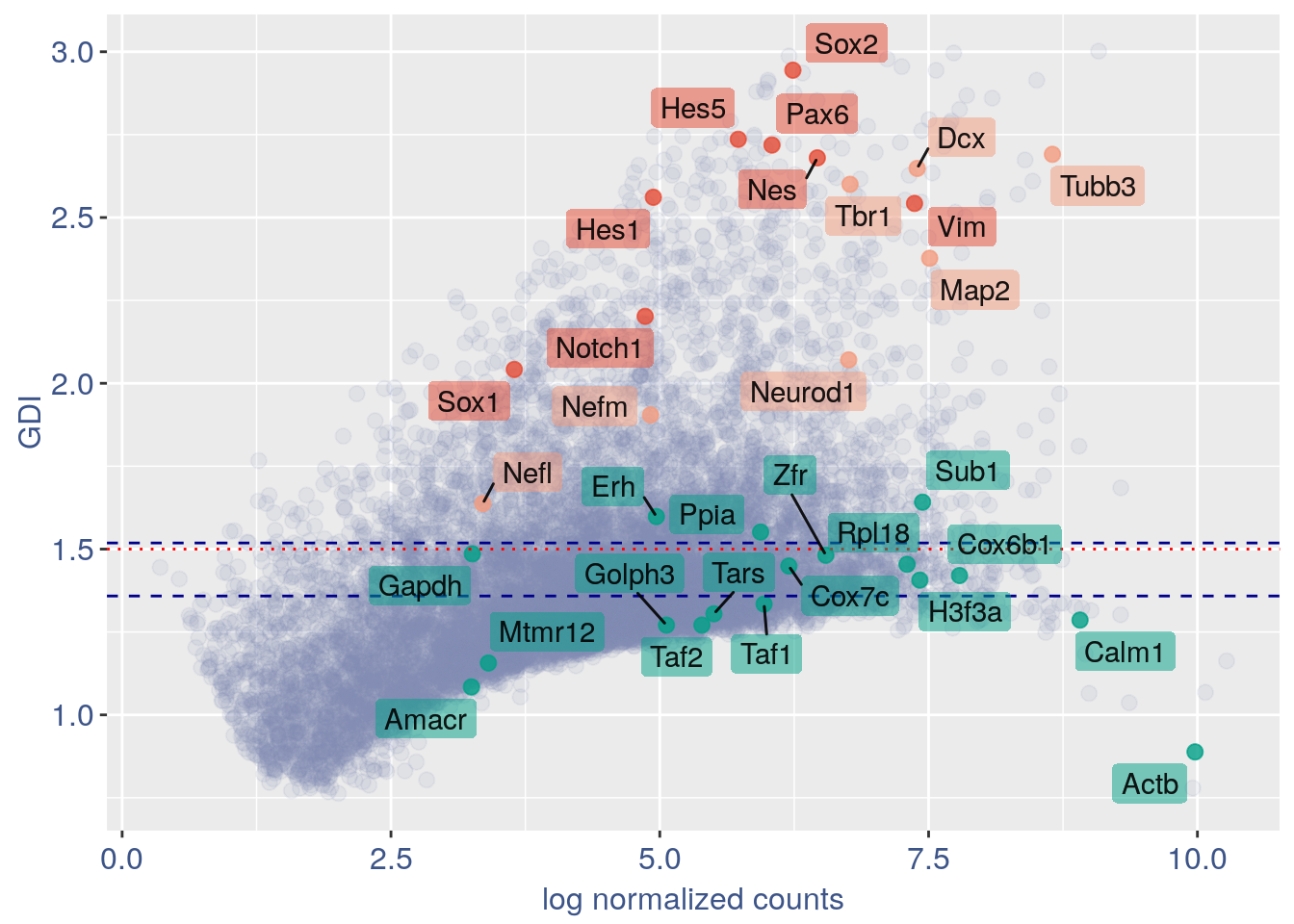
3.3 Heatmaps with cleaning
For the Gene Pair Analysis, we can plot an heatmap with the coex values between two genes sets. To do so we need to define, in a list, the different gene sets (list.genes). Then in the function parameter sets we can decide which sets need to be considered (in the example from 1 to 3). In the condition parameter we should insert an array with each file name prefix to be considered (in the example, the file names is “E13_cortex_clean”).
list.genes = list(Ref.col = PNGs, NPGs = NPGs,
    Const. = hk)

plot_heatmap(df_genes = list.genes, sets = c(1:3),
    conditions = "E13_cortex_clean", dir = "Data/")
#> [1] "plot heatmap"
#> [1] "Loading condition E13_cortex_clean"
#> [1] "Map2"    "Tubb3"   "Neurod1" "Nefm"    "Nefl"    "Dcx"     "Tbr1"
#> [1] "Get p-values on a set of genes on columns on a set of genes on rows"
#> [1] "Using function S"
#> [1] "function to generate S "
#> [1] "Ref.col"
#> [1] "NPGs"
#> [1] "Const."
#> [1] "min coex: -0.0121911229941534 max coex 0.00944576864330662"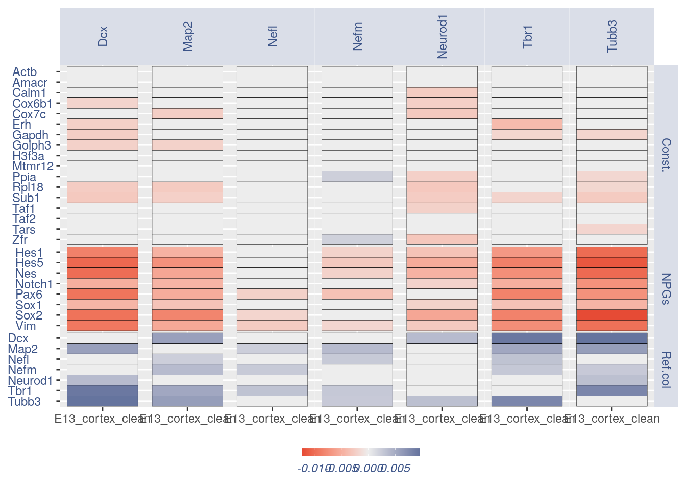
3.4 Heatmaps without cleaning
list.genes = list(Ref.col = PNGs, NPGs = NPGs,
    Const. = hk)

plot_heatmap(df_genes = list.genes, sets = c(1:3),
    conditions = "E13_cortex", dir = "Data/")
#> [1] "plot heatmap"
#> [1] "Loading condition E13_cortex"
#> [1] "Map2"    "Tubb3"   "Neurod1" "Nefm"    "Nefl"    "Dcx"     "Tbr1"
#> [1] "Get p-values on a set of genes on columns on a set of genes on rows"
#> [1] "Using function S"
#> [1] "function to generate S "
#> [1] "Ref.col"
#> [1] "NPGs"
#> [1] "Const."
#> [1] "min coex: -0.0120306783883114 max coex 0.00921583325423012"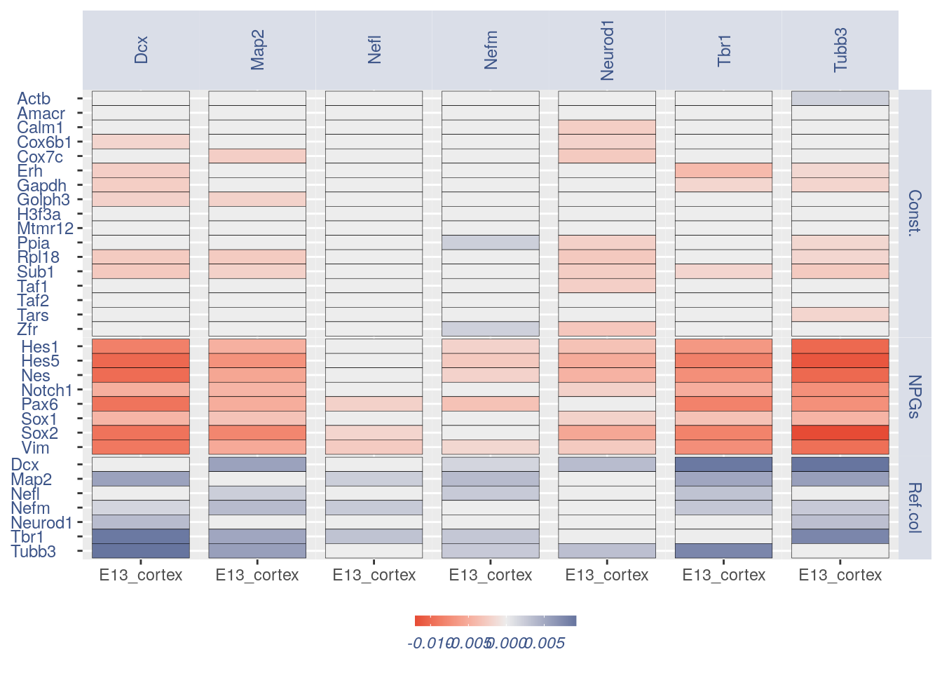
print(sessionInfo())
#> R version 4.0.4 (2021-02-15)
#> Platform: x86_64-pc-linux-gnu (64-bit)
#> Running under: Ubuntu 18.04.5 LTS
#>
#> Matrix products: default
#> BLAS:   /usr/lib/x86_64-linux-gnu/openblas/libblas.so.3
#> LAPACK: /usr/lib/x86_64-linux-gnu/libopenblasp-r0.2.20.so
#>
#> locale:
#>  [1] LC_CTYPE=en_US.UTF-8       LC_NUMERIC=C
#>  [3] LC_TIME=en_US.UTF-8        LC_COLLATE=en_US.UTF-8
#>  [5] LC_MONETARY=en_US.UTF-8    LC_MESSAGES=en_US.UTF-8
#>  [7] LC_PAPER=en_US.UTF-8       LC_NAME=C
#>  [9] LC_ADDRESS=C               LC_TELEPHONE=C
#> [11] LC_MEASUREMENT=en_US.UTF-8 LC_IDENTIFICATION=C
#>
#> attached base packages:
#> [1] stats     graphics  grDevices utils     datasets  methods   base
#>
#> other attached packages:
#> [1] ggrepel_0.9.1     ggplot2_3.3.3     Matrix_1.3-2      data.table_1.14.0
#> [5] COTAN_0.1.0
#>
#> loaded via a namespace (and not attached):
#>  [1] sass_0.3.1           tidyr_1.1.2          jsonlite_1.7.2
#>  [4] R.utils_2.10.1       bslib_0.2.4          assertthat_0.2.1
#>  [7] highr_0.8            stats4_4.0.4         yaml_2.2.1
#> [10] pillar_1.5.1         lattice_0.20-41      glue_1.4.2
#> [13] reticulate_1.18      digest_0.6.27        RColorBrewer_1.1-2
#> [16] colorspace_2.0-0     cowplot_1.1.1        htmltools_0.5.1.1
#> [19] R.oo_1.24.0          pkgconfig_2.0.3      GetoptLong_1.0.5
#> [22] purrr_0.3.4          scales_1.1.1         tibble_3.1.0
#> [25] generics_0.1.0       farver_2.1.0         IRanges_2.24.1
#> [28] ellipsis_0.3.1       withr_2.4.1          BiocGenerics_0.36.0
#> [31] magrittr_2.0.1       crayon_1.4.0         evaluate_0.14
#> [34] R.methodsS3_1.8.1    fansi_0.4.2          Cairo_1.5-12.2
#> [37] tools_4.0.4          GlobalOptions_0.1.2  formatR_1.8
#> [40] lifecycle_1.0.0      matrixStats_0.58.0   ComplexHeatmap_2.6.2
#> [43] basilisk.utils_1.2.2 stringr_1.4.0        S4Vectors_0.28.1
#> [46] munsell_0.5.0        cluster_2.1.1        compiler_4.0.4
#> [49] jquerylib_0.1.3      rlang_0.4.10         grid_4.0.4
#> [52] rjson_0.2.20         rappdirs_0.3.3       circlize_0.4.12
#> [55] labeling_0.4.2       rmarkdown_2.7        basilisk_1.2.1
#> [58] gtable_0.3.0         DBI_1.1.1            R6_2.5.0
#> [61] knitr_1.31           dplyr_1.0.4          utf8_1.2.1
#> [64] clue_0.3-58          filelock_1.0.2       shape_1.4.5
#> [67] stringi_1.5.3        parallel_4.0.4       Rcpp_1.0.6
#> [70] vctrs_0.3.6          png_0.1-7            tidyselect_1.1.0
#> [73] xfun_0.22