E11.5 cortex
library(COTAN)
library(data.table)
library(Matrix)
library(ggrepel)
#> Loading required package: ggplot2
# library(latex2exp)
mycolours <- c(A = "#8491B4B2", B = "#E64B35FF")
my_theme = theme(axis.text.x = element_text(size = 14,
angle = 0, hjust = 0.5, vjust = 0.5,
face = "plain", colour = "#3C5488FF"),
axis.text.y = element_text(size = 14,
angle = 0, hjust = 0, vjust = 0.5,
face = "plain", colour = "#3C5488FF"),
axis.title.x = element_text(size = 14,
angle = 0, hjust = 0.5, vjust = 0,
face = "plain", colour = "#3C5488FF"),
axis.title.y = element_text(size = 14,
angle = 90, hjust = 0.5, vjust = 0.5,
face = "plain", colour = "#3C5488FF"))data = as.data.frame(fread(paste(data_dir,
"GSM2861510_E115_Only_Cortical_Cells_DGE.txt.gz",
sep = "/")))
data = as.data.frame(data)
rownames(data) = data$V1
data = data[, 2:ncol(data)]
data[1:10, 1:10]
#> ATGTAGTACCGA TCAACTTCATAT ATGAAAGACCAT CCGTACCGCGTA ATCACCCGTGTT
#> 0610005C13Rik 0 0 0 0 0
#> 0610007N19Rik 0 0 0 0 3
#> 0610007P14Rik 0 0 2 2 1
#> 0610009B22Rik 2 0 0 2 0
#> 0610009D07Rik 4 6 5 5 3
#> 0610009E02Rik 0 0 0 0 0
#> 0610009L18Rik 0 0 1 1 0
#> 0610009O20Rik 0 2 0 0 0
#> 0610010F05Rik 0 0 2 0 1
#> 0610010K14Rik 0 0 0 0 0
#> ATCTCCGCACGT CCCTTCTCCTAC AATCAGTTGCTT AGTAAAGGACTT CTGCGCTTACCT
#> 0610005C13Rik 0 0 0 0 0
#> 0610007N19Rik 0 1 2 0 0
#> 0610007P14Rik 2 0 3 1 0
#> 0610009B22Rik 1 0 1 0 1
#> 0610009D07Rik 1 4 2 5 7
#> 0610009E02Rik 0 1 0 0 0
#> 0610009L18Rik 0 1 0 0 0
#> 0610009O20Rik 0 1 0 1 0
#> 0610010F05Rik 5 1 1 0 0
#> 0610010K14Rik 0 0 0 0 0Define a directory where the ouput will be stored.
1 Analytical pipeline
Initialize the COTAN object with the row count table and the metadata for the experiment.
obj = new("scCOTAN", raw = data)
obj = initRaw(obj, GEO = "GSM2861510", sc.method = "DropSeq",
    cond = "mouse cortex E11.5")
#> [1] "Initializing S4 object"
Now we can start the cleaning. Analysis requires and starts from a matrix of raw UMI counts after removing possible cell doublets or multiplets and low quality or dying cells (with too high mtRNA percentage, easily done with Seurat or other tools).
If we do not want to consider the mitochondrial genes we can remove them before starting the analysis.
genes_to_rem = rownames(obj@raw[grep("^mt",
    rownames(obj@raw)), ])  #genes to remove : mithocondrial
obj@raw = obj@raw[!rownames(obj@raw) %in%
    genes_to_rem, ]
cells_to_rem = colnames(obj@raw[which(colSums(obj@raw) ==
    0)])
obj@raw = obj@raw[, !colnames(obj@raw) %in%
    cells_to_rem]
We want also to define a prefix to identify the sample.
t = "E11_cortex_clean"

print(paste("Condition ", t, sep = ""))
#> [1] "Condition E11_cortex_clean"
#--------------------------------------
n_cells = length(colnames(obj@raw))
print(paste("n cells", n_cells, sep = " "))
#> [1] "n cells 1418"

n_it = 1

# obj@raw = obj@raw[rownames(cells),
# colnames(cells)]
2 Data cleaning
First, we create the directory to store all information regarding the data cleaning.
if (!file.exists(out_dir)) {
    dir.create(file.path(out_dir))
}

if (!file.exists(paste(out_dir, "cleaning",
    sep = ""))) {
    dir.create(file.path(out_dir, "cleaning"))
}
ttm = clean(obj)
#> [1] "Start estimation mu with linear method"
#> [1] 12549 1418
#> rowname CAGAGCTTTACG GCCCCTCACGAT CGGCAACTATCA GGCGGAGGCGTA
#> 5167 Hbb-y 174.578095 340.178647 224.552985 329.057856
#> 5163 Hba-x 112.695946 117.536808 129.919941 171.739359
#> 5162 Hba-a1 44.776514 149.181333 65.761945 60.305424
#> 5164 Hbb-bh1 57.354187 24.863556 48.118497 73.415299
#> 5354 Hnrnpa2b1 8.049710 19.212747 14.435549 11.798887
#> 5417 Hsp90ab1 13.583886 14.692101 9.623699 7.865925
#> 5166 Hbb-bt 1.509321 13.561939 6.415800 19.664812
#> 4081 Fth1 9.559031 13.561939 6.415800 10.487900
#> 6294 Malat1 3.521748 10.171455 12.831599 3.932962
#> 682 Actb 5.031069 2.260323 8.019749 11.798887
#> 9342 Rps9 11.571459 9.041293 4.811850 3.932962
#> 11448 Tubb5 6.037283 3.390485 6.415800 5.243950
#> 9223 Rpl13a 9.559031 7.911131 4.811850 3.932962
#> 9251 Rpl32 9.055924 11.301616 3.207900 11.798887
#> 11990 Ybx1 10.565245 10.171455 4.811850 2.621975
#> TGTTAGCGCGGA ATGGATCTCATT
#> 5167 131.348618 509.114655
#> 5163 76.043937 295.226249
#> 5162 93.326650 96.400408
#> 5164 3.456543 156.650663
#> 5354 6.913085 0.000000
#> 5417 3.456543 9.037538
#> 5166 13.826170 3.012513
#> 4081 3.456543 12.050051
#> 6294 13.826170 6.025025
#> 682 10.369628 12.050051
#> 9342 10.369628 6.025025
#> 11448 17.282713 6.025025
#> 9223 6.913085 9.037538
#> 9251 3.456543 3.012513
#> 11990 10.369628 3.012513
obj = ttm$object
ttm$pca.cell.2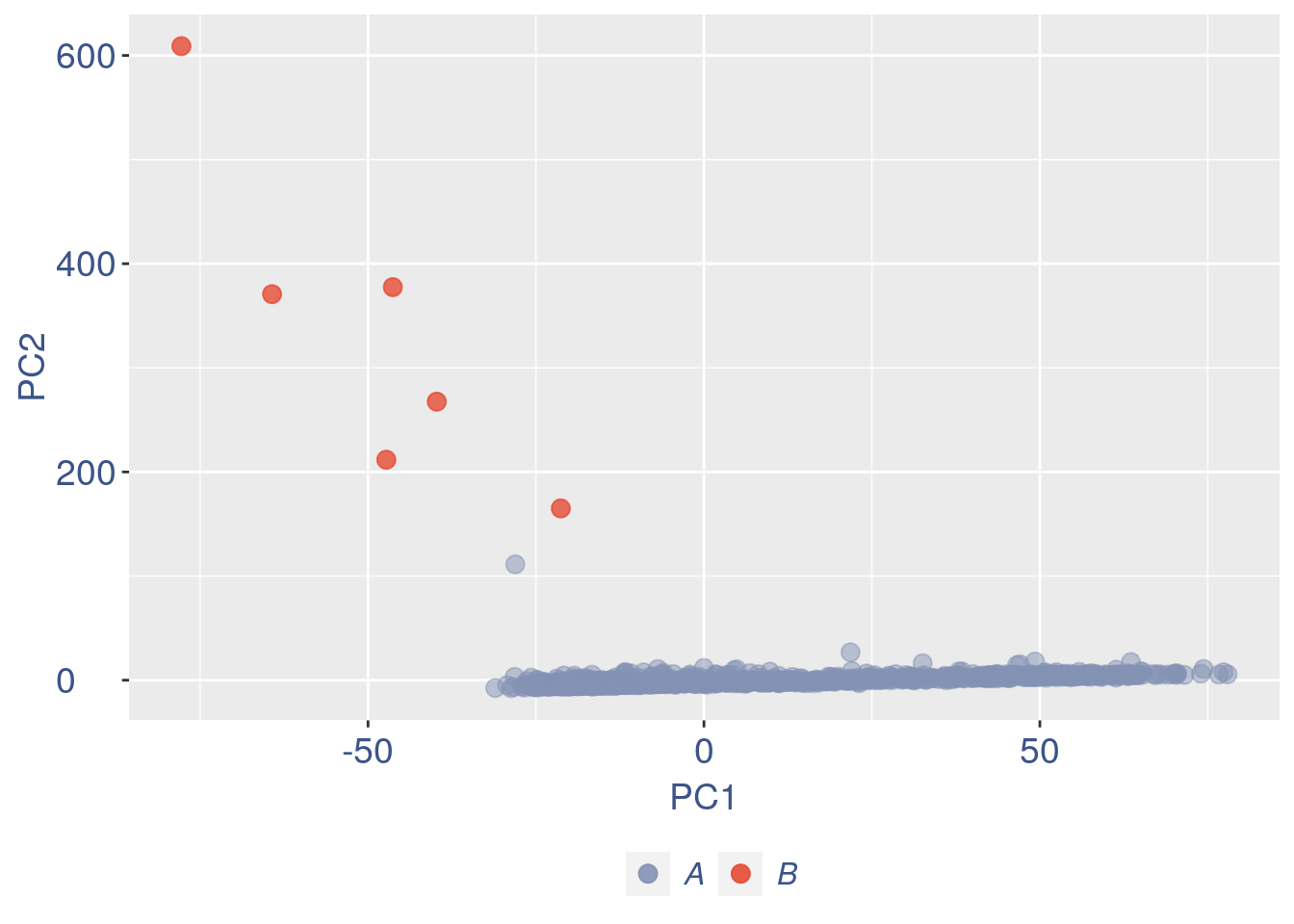
Run this when B cells need to be removed.
pdf(paste(out_dir, "cleaning/", t, "_", n_it,
    "_plots_before_cells_exlusion.pdf", sep = ""))
ttm$pca.cell.2
ggplot(ttm$D, aes(x = n, y = means)) + geom_point() +
    geom_text_repel(data = subset(ttm$D,
        n > (max(ttm$D$n) - 15)), aes(n,
        means, label = rownames(ttm$D[ttm$D$n >
            (max(ttm$D$n) - 15), ])), nudge_y = 0.05,
        nudge_x = 0.05, direction = "x",
        angle = 90, vjust = 0, segment.size = 0.2) +
    ggtitle("B cell group genes mean expression") +
    my_theme + theme(plot.title = element_text(color = "#3C5488FF",
    size = 20, face = "italic", vjust = -5,
    hjust = 0.02))
dev.off()
#> png
#>   2

if (length(ttm$cl1) < length(ttm$cl2)) {
    to_rem = ttm$cl1
} else {
    to_rem = ttm$cl2
}
n_it = n_it + 1
obj@raw = obj@raw[, !colnames(obj@raw) %in%
    to_rem]
# obj@raw = obj@raw[rownames(obj@raw)
# %in% rownames(cells),colnames(obj@raw)
# %in% colnames(cells)]
gc()
#>             used  (Mb) gc trigger   (Mb)  max used   (Mb)
#> Ncells   3734773 199.5    6027515  322.0   6027515  322.0
#> Vcells 120442987 919.0  206449142 1575.1 171973003 1312.1

ttm = clean(obj)
#> [1] "Start estimation mu with linear method"
#> [1] 12543  1412
#>         rowname GCATATTACGCC TGAGAGCGAAGG
#> 6291     Malat1   278.591783   350.707493
#> 7296       Nnat    49.370696    11.888390
#> 6513       Meg3     3.526478    53.497753
#> 1353       Atrx    10.579435    23.776779
#> 11430    Tuba1a    28.211826     5.944195
#> 11104    Tmsb10    28.211826     0.000000
#> 839       Akap9     0.000000    23.776779
#> 681        Actb    17.632391     5.944195
#> 6230     Luc7l3     3.526478    17.832584
#> 7618      Pa2g4     3.526478    17.832584
#> 5351  Hnrnpa2b1    21.158870     0.000000
#> 4122      G3bp2     7.052957    11.888390
#> 11945      Xist     7.052957    11.888390
#> 2313      Ckap4     0.000000    17.832584
#> 2380       Cmip     0.000000    17.832584
# ttm = clean.sqrt(obj, cells)
obj = ttm$object

ttm$pca.cell.2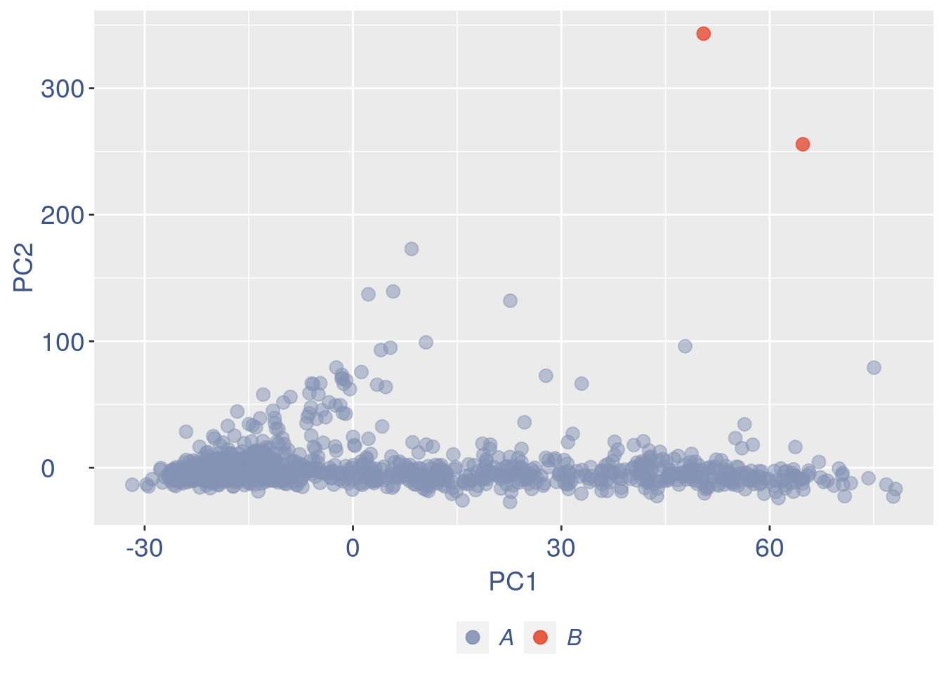
#> png
#>   2
#>             used  (Mb) gc trigger   (Mb)  max used   (Mb)
#> Ncells   3734996 199.5    6027515  322.0   6027515  322.0
#> Vcells 123175645 939.8  297462764 2269.5 297462305 2269.5
#> [1] "Start estimation mu with linear method"
#> [1] 12539  1410
#>       rowname GTAGCCAATCAA GCACACGCCTCA TCGATGCTCCGG CGGCTGTTCCGC TATATAAGTATC
#> 6289   Malat1   137.826998   139.765012   182.524171    96.726725   136.543974
#> 7293     Nnat     0.000000     0.000000     0.000000    73.967496     5.461759
#> 11942    Xist    13.338097    15.529446     0.000000    11.379615    10.923518
#> 11427  Tuba1a     4.446032     0.000000     0.000000    34.138844    10.923518
#> 11981    Ybx1     8.892064     7.764723     4.148277    11.379615    16.385277
#> 5646    Islr2     0.000000     0.000000     4.148277    28.449037    10.923518
#> 9335     Rps9     0.000000    11.647084    12.444830     5.689807    10.923518
#> 9692   Sfrs18     8.892064    23.294169     4.148277     0.000000     0.000000
#> 8624    Ptprs     0.000000     7.764723     0.000000    17.069422    10.923518
#> 10222     Son     8.892064    11.647084     4.148277     0.000000    10.923518
#> 11439   Tubb5     0.000000     7.764723    16.593106     0.000000    10.923518
#> 8895    Rbm25    13.338097     0.000000     4.148277    11.379615     5.461759
#> 9309    Rps26     0.000000    19.411807     8.296553     5.689807     0.000000
#> 1502    Baz1b     8.892064     7.764723     8.296553     5.689807     0.000000
#> 6510     Meg3     4.446032     0.000000    24.889660     0.000000     0.000000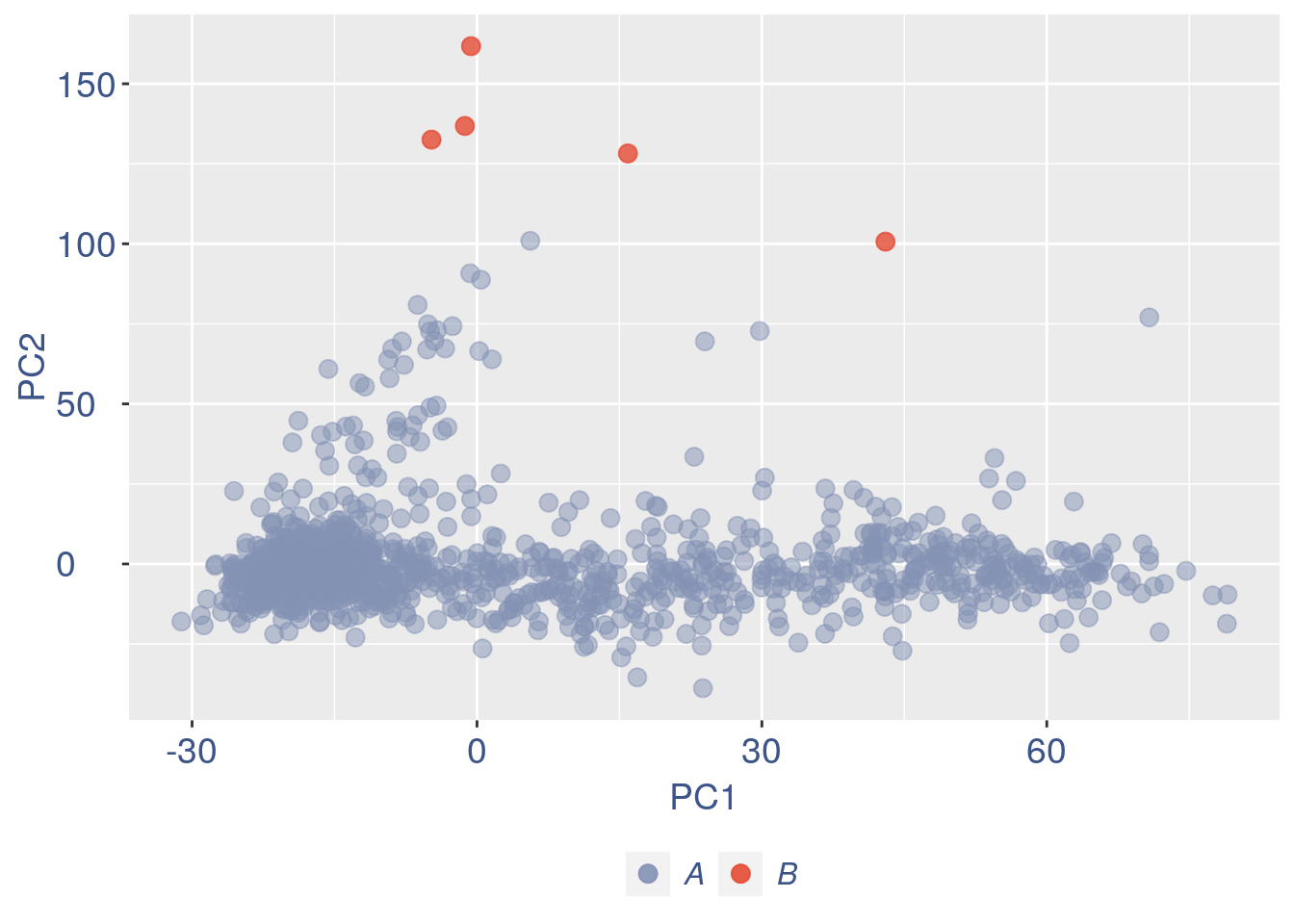
Run this only in the last iteration, instead the previous code, when B cells group has not to be removed.
pdf(paste(out_dir, "cleaning/", t, "_", n_it,
    "_plots_before_cells_exlusion.pdf", sep = ""))
ttm$pca.cell.2
ggplot(ttm$D, aes(x = n, y = means)) + geom_point() +
    geom_text_repel(data = subset(ttm$D,
        n > (max(ttm$D$n) - 15)), aes(n,
        means, label = rownames(ttm$D[ttm$D$n >
            (max(ttm$D$n) - 15), ])), nudge_y = 0.05,
        nudge_x = 0.05, direction = "x",
        angle = 90, vjust = 0, segment.size = 0.2) +
    ggtitle(label = "B cell group genes mean expression",
        subtitle = " - B group NOT removed -") +
    my_theme + theme(plot.title = element_text(color = "#3C5488FF",
    size = 20, face = "italic", vjust = -10,
    hjust = 0.02), plot.subtitle = element_text(color = "darkred",
    vjust = -15, hjust = 0.01))

dev.off()
#> png
#>   2
To color the pca based on nu_j (so the cells’ efficiency)
nu_est = round(obj@nu, digits = 7)

plot.nu <- ggplot(ttm$pca_cells, aes(x = PC1,
    y = PC2, colour = log(nu_est)))

plot.nu = plot.nu + geom_point(size = 1,
    alpha = 0.8) + scale_color_gradient2(low = "#E64B35B2",
    mid = "#4DBBD5B2", high = "#3C5488B2",
    midpoint = log(mean(nu_est)), name = "ln (nu)") +
    ggtitle("Cells PCA coloured by cells efficiency") +
    my_theme + theme(plot.title = element_text(color = "#3C5488FF",
    size = 20), legend.title = element_text(color = "#3C5488FF",
    size = 14, face = "italic"), legend.text = element_text(color = "#3C5488FF",
    size = 11), legend.key.width = unit(2,
    "mm"), legend.position = "right")

pdf(paste(out_dir, "cleaning/", t, "_plots_PCA_efficiency_colored.pdf",
    sep = ""))
plot.nu
dev.off()
#> png
#>   2

plot.nu
The next part is use to remove the cells with efficiency too low.
nu_df = data.frame(nu = sort(obj@nu), n = c(1:length(obj@nu)))

ggplot(nu_df, aes(x = n, y = nu)) + geom_point(colour = "#8491B4B2",
    size = 1) + my_theme  #+ ylim(0,1) + xlim(0,70)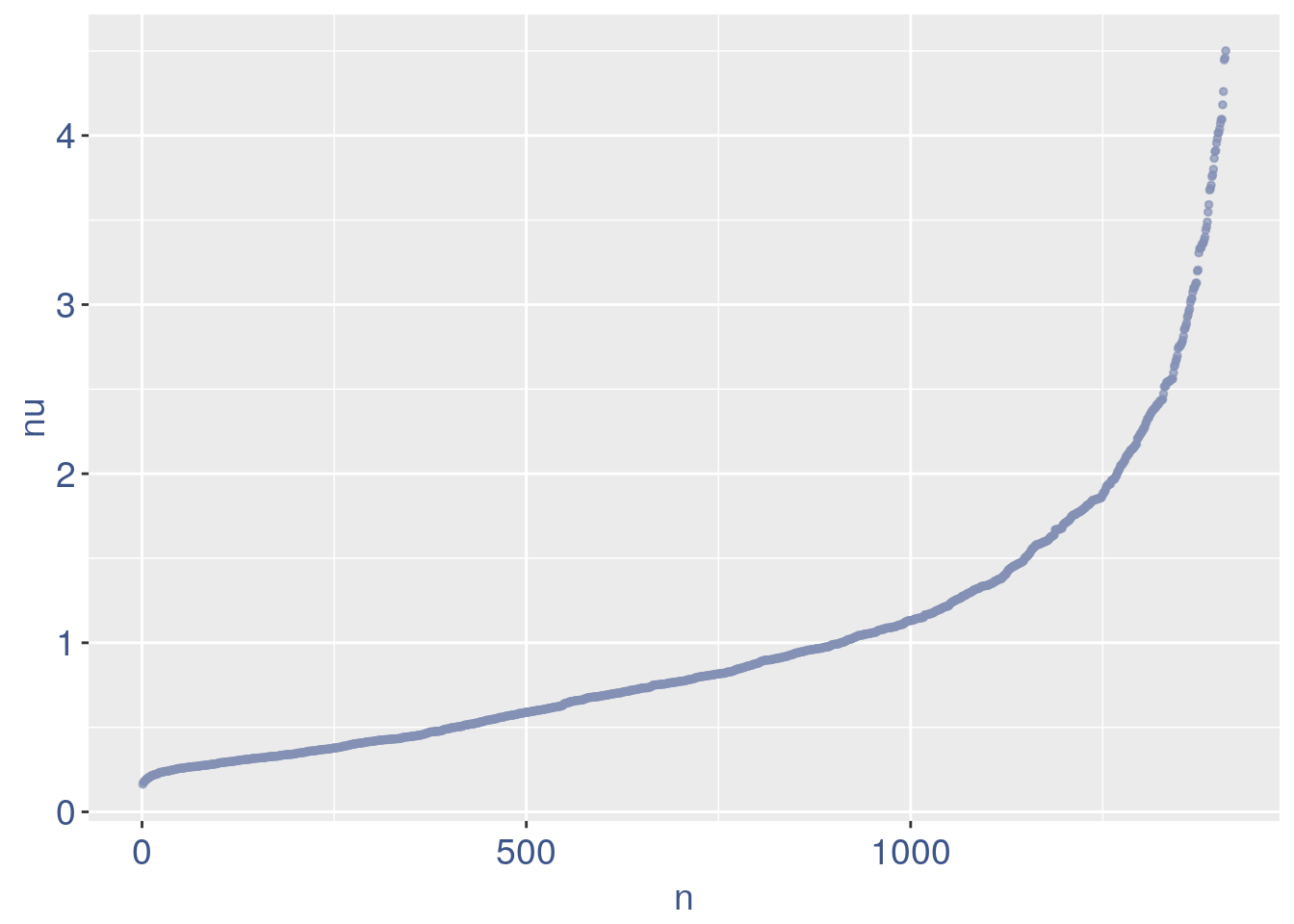
We can zoom on the smalest values and, if we detect a clear elbow, we can decide to remove the cells.
yset = 0.21  #threshold to remove low UDE cells
plot.ude <- ggplot(nu_df, aes(x = n, y = nu)) +
    geom_point(colour = "#8491B4B2", size = 1) +
    my_theme + ylim(0, 0.4) + xlim(0, 200) +
    geom_hline(yintercept = yset, linetype = "dashed",
        color = "darkred") + annotate(geom = "text",
    x = 500, y = 0.5, label = paste("to remove cells with nu < ",
        yset, sep = " "), color = "darkred",
    size = 4.5)


pdf(paste(out_dir, "cleaning/", t, "_plots_efficiency.pdf",
    sep = ""))
plot.ude
dev.off()
#> png
#>   2

plot.ude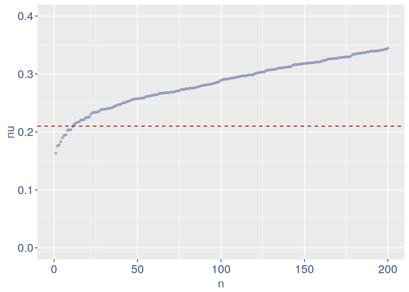
We also save the defined threshold in the metadata and re run the estimation
obj@meta[(nrow(obj@meta) + 1), 1:2] = c("Threshold low UDE cells:",
    yset)

to_rem = rownames(nu_df[which(nu_df$nu <
    yset), ])

obj@raw = obj@raw[, !colnames(obj@raw) %in%
    to_rem]
Repeat the estimation after the cells are removed
ttm = clean(obj)
#> [1] "Start estimation mu with linear method"
#> [1] 12537  1399
#>       rowname TCCCTCTTATAC GTAGCCAATCAA GCACACGCCTCA TCGATGCTCCGG CCCATCCCGGGC
#> 6288   Malat1    98.595685   138.703643   140.653984   183.685111   103.892147
#> 11940    Xist    26.889732    13.422933    15.628220     0.000000     0.000000
#> 9691   Sfrs18     8.963244     8.948622    23.442331     4.174662     4.155686
#> 6227   Luc7l3    13.444866    13.422933     7.814110     4.174662     8.311372
#> 11979    Ybx1     0.000000     8.948622     7.814110     4.174662    20.778429
#> 9334     Rps9     4.481622     0.000000    11.721165    12.523985    12.467058
#> 10221     Son    13.444866     8.948622    11.721165     4.174662     0.000000
#> 9256    Rpl41     8.963244     0.000000     3.907055    16.698646     8.311372
#> 6509     Meg3     0.000000     4.474311     0.000000    25.047970     8.311372
#> 9633   Serbp1    13.444866     0.000000    11.721165     4.174662     8.311372
#> 681      Actb    13.444866     0.000000     0.000000     4.174662    16.622744
#> 7615   Pabpc1     8.963244     0.000000     7.814110     0.000000    16.622744
#> 10366   Srrm2    17.926488     4.474311     7.814110     0.000000     0.000000
#> 5559   Incenp    13.444866     8.948622     7.814110     0.000000     0.000000
#> 9215   Rpl13a     8.963244     4.474311     7.814110     4.174662     4.155686
obj = ttm$object
ttm$pca.cell.2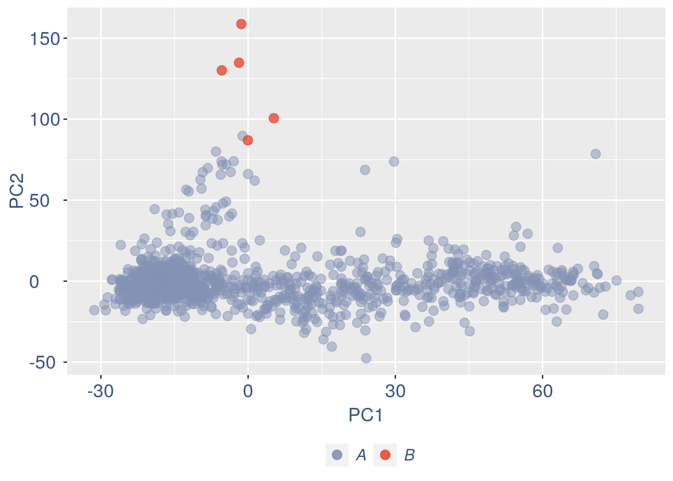
Just to check again, we plot the final efficiency colored PCA
nu_est = round(obj@nu, digits = 7)
plot.nu <- ggplot(ttm$pca_cells, aes(x = PC1,
    y = PC2, colour = log(nu_est)))
plot.nu = plot.nu + geom_point(size = 2,
    alpha = 0.8) + scale_color_gradient2(low = "#E64B35B2",
    mid = "#4DBBD5B2", high = "#3C5488B2",
    midpoint = log(mean(nu_est)), name = "ln(nu)") +
    ggtitle("Cells PCA coloured by cells efficiency: last") +
    my_theme + theme(plot.title = element_text(color = "#3C5488FF",
    size = 20), legend.title = element_text(color = "#3C5488FF",
    size = 14, face = "italic"), legend.text = element_text(color = "#3C5488FF",
    size = 11), legend.key.width = unit(2,
    "mm"), legend.position = "right")

pdf(paste(out_dir, "cleaning/", t, "_plots_PCA_efficiency_colored_FINAL.pdf",
    sep = ""))
plot.nu
dev.off()
#> png
#>   2

plot.nu
COTAN analysis: in this part all the contingency tables are computed and used to get the statistics (S). To storage efficiency of all the observed tables only the yes_yes is stored. Note that if will be necessary re-coputing the yes-yes table, the yes-yes table should be cancelled before running cotan_analysis.
COEX evaluation and storing
saveRDS(obj, file = paste(out_dir, t, ".cotan.RDS",
    sep = ""))

obj = get.coex(obj)

# saving the structure
saveRDS(obj, file = paste(out_dir, t, ".cotan.RDS",
    sep = ""))
Automatic data elaboration (without cleaning)
obj2 = automatic.COTAN.object.creation(df = data,
    GEO = "GSM2861510", sc.method = "Drop-seq",
    cond = "E11_cortex", out_dir = "Data/")
#> [1] "Initializing S4 object"
#> [1] "Condition E11_cortex"
#> [1] "n cells 1418"
#> [1] "Start estimation mu with linear method"
#> [1] 12549  1418
#>         rowname CAGAGCTTTACG GCCCCTCACGAT CGGCAACTATCA GGCGGAGGCGTA
#> 5167      Hbb-y   174.578095   340.178647   224.552985   329.057856
#> 5163      Hba-x   112.695946   117.536808   129.919941   171.739359
#> 5162     Hba-a1    44.776514   149.181333    65.761945    60.305424
#> 5164    Hbb-bh1    57.354187    24.863556    48.118497    73.415299
#> 5354  Hnrnpa2b1     8.049710    19.212747    14.435549    11.798887
#> 5417   Hsp90ab1    13.583886    14.692101     9.623699     7.865925
#> 5166     Hbb-bt     1.509321    13.561939     6.415800    19.664812
#> 4081       Fth1     9.559031    13.561939     6.415800    10.487900
#> 6294     Malat1     3.521748    10.171455    12.831599     3.932962
#> 682        Actb     5.031069     2.260323     8.019749    11.798887
#> 9342       Rps9    11.571459     9.041293     4.811850     3.932962
#> 11448     Tubb5     6.037283     3.390485     6.415800     5.243950
#> 9223     Rpl13a     9.559031     7.911131     4.811850     3.932962
#> 9251      Rpl32     9.055924    11.301616     3.207900    11.798887
#> 11990      Ybx1    10.565245    10.171455     4.811850     2.621975
#>       TGTTAGCGCGGA ATGGATCTCATT
#> 5167    131.348618   509.114655
#> 5163     76.043937   295.226249
#> 5162     93.326650    96.400408
#> 5164      3.456543   156.650663
#> 5354      6.913085     0.000000
#> 5417      3.456543     9.037538
#> 5166     13.826170     3.012513
#> 4081      3.456543    12.050051
#> 6294     13.826170     6.025025
#> 682      10.369628    12.050051
#> 9342     10.369628     6.025025
#> 11448    17.282713     6.025025
#> 9223      6.913085     9.037538
#> 9251      3.456543     3.012513
#> 11990    10.369628     3.012513
#> [1] "Cotan analysis function started"
#> [1] "cotan analysis"
#> [1] "mu estimator creation"
#> [1] "save effective constitutive genes"
#> [1] "start a minimization"
#> [1] "Next gene: Capn2 number 1810"
#> [1] "Next gene: Fam83h number 3820"
#> [1] "Next gene: Kidins220 number 5830"
#> [1] "Next gene: Pds5a number 7840"
#> [1] "Next gene: Slc18b1 number 9850"
#> [1] "Next gene: Wdr26 number 11860"
#> [1] "Final trance!"
#> [1] "a min: -0.0564117431640625 | a max 371.625 | negative a %: 18.2962785879353"
#> [1] "Only analysis time 0.909146149953206"
#> [1] "Cotan coex estimation started"
#> [1] "coex dataframe creation"
#> [1] "Generating contingency tables for observed data"
#> [1] "creation of observed yes/yes contingency table"
#> [1] "mu estimator creation"
#> [1] "expected contingency tables creation"
#> [1] "The distance between estimated n of zeros and observed number of zero is 0.0593550958424397 over 12549"
#> [1] "Done"
#> [1] "coex estimation"
#> [1] "Diagonal coex values substituted with 0"
#> [1] "Total time 2.62279897928238"
#> [1] "Only coex time 1.57342616717021"
#> [1] "Saving elaborated data locally at Data/E11_cortex.cotan.RDS"
3 Analysis of the elaborated data
In this case the test possible macroscopic differences between cleaned and not cleaned data.
The initial cell number was:
obj = readRDS(paste(out_dir, t, ".cotan.RDS",
    sep = ""))
obj@meta
#>                         V1                 V2
#> 1                     GEO:         GSM2861510
#> 2         scRNAseq method:            DropSeq
#> 3    starting n. of cells:               1418
#> 4        Condition sample: mouse cortex E11.5
#> 5 Threshold low UDE cells:               0.21
While the final number of cells was:
So were removed:
cells
3.1 GDI with cleaning
quant.p = get.GDI(obj)
#> [1] "function to generate GDI dataframe"
#> [1] "Using S"
#> [1] "function to generate S "

head(quant.p)
#>               sum.raw.norm      GDI exp.cells
#> 0610007N19Rik     4.779046 1.511822  7.219442
#> 0610007P14Rik     5.747081 1.604336 19.370979
#> 0610009B22Rik     5.938677 1.327618 20.657613
#> 0610009D07Rik     7.334895 1.554625 56.683345
#> 0610009E02Rik     3.591232 1.314033  2.358828
#> 0610009L18Rik     4.115833 1.282979  3.359543
In the third column of this data frame is reported the percentage of cells expressing the gene.
NPGs = c("Nes", "Vim", "Sox2", "Sox1", "Notch1",
    "Hes1", "Hes5", "Pax6")  #,'Hes3'
PNGs = c("Map2", "Tubb3", "Neurod1", "Nefm",
    "Nefl", "Dcx", "Tbr1")
hk = c("Calm1", "Cox6b1", "Ppia", "Rpl18",
    "Cox7c", "Erh", "H3f3a", "Taf1", "Taf2",
    "Gapdh", "Actb", "Golph3", "Mtmr12",
    "Zfr", "Sub1", "Tars", "Amacr")

text.size = 12

quant.p$highlight = with(quant.p, ifelse(rownames(quant.p) %in%
    NPGs, "NPGs", ifelse(rownames(quant.p) %in%
    hk, "Constitutive", ifelse(rownames(quant.p) %in%
    PNGs, "PNGs", "normal"))))

textdf <- quant.p[rownames(quant.p) %in%
    c(NPGs, hk, PNGs), ]
mycolours <- c(Constitutive = "#00A087FF",
    NPGs = "#E64B35FF", PNGs = "#F39B7FFF",
    normal = "#8491B4B2")
f1 = ggplot(subset(quant.p, highlight ==
    "normal"), aes(x = sum.raw.norm, y = GDI)) +
    geom_point(alpha = 0.1, color = "#8491B4B2",
        size = 2.5)
GDI_plot = f1 + geom_point(data = subset(quant.p,
    highlight != "normal"), aes(x = sum.raw.norm,
    y = GDI, colour = highlight), size = 2.5,
    alpha = 0.8) + geom_hline(yintercept = quantile(quant.p$GDI)[4],
    linetype = "dashed", color = "darkblue") +
    geom_hline(yintercept = quantile(quant.p$GDI)[3],
        linetype = "dashed", color = "darkblue") +
    geom_hline(yintercept = 1.5, linetype = "dotted",
        color = "red", size = 0.5) + scale_color_manual("Status",
    values = mycolours) + scale_fill_manual("Status",
    values = mycolours) + xlab("log normalized counts") +
    ylab("GDI") + geom_label_repel(data = textdf,
    aes(x = sum.raw.norm, y = GDI, label = rownames(textdf),
        fill = highlight), label.size = NA,
    alpha = 0.5, direction = "both", na.rm = TRUE,
    seed = 1234) + geom_label_repel(data = textdf,
    aes(x = sum.raw.norm, y = GDI, label = rownames(textdf)),
    label.size = NA, segment.color = "black",
    segment.size = 0.5, direction = "both",
    alpha = 0.8, na.rm = TRUE, fill = NA,
    seed = 1234) + theme(axis.text.x = element_text(size = text.size,
    angle = 0, hjust = 0.5, vjust = 0.5,
    face = "plain", colour = "#3C5488FF"),
    axis.text.y = element_text(size = text.size,
        angle = 0, hjust = 0, vjust = 0.5,
        face = "plain", colour = "#3C5488FF"),
    axis.title.x = element_text(size = text.size,
        angle = 0, hjust = 0.5, vjust = 0,
        face = "plain", colour = "#3C5488FF"),
    axis.title.y = element_text(size = text.size,
        angle = 90, hjust = 0.5, vjust = 0.5,
        face = "plain", colour = "#3C5488FF"),
    legend.title = element_blank(), legend.text = element_text(color = "#3C5488FF",
        face = "italic"), legend.position = "bottom")  # titl)
legend <- cowplot::get_legend(GDI_plot)
GDI_plot = GDI_plot + theme(legend.position = "none")
GDI_plot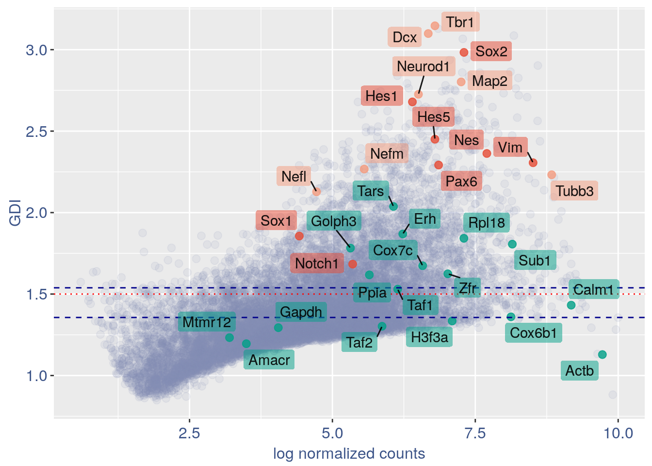
3.2 GDI without cleaning
quant.p = get.GDI(obj2)
#> [1] "function to generate GDI dataframe"
#> [1] "Using S"
#> [1] "function to generate S "

head(quant.p)
#>               sum.raw.norm      GDI exp.cells
#> 0610007N19Rik     4.781870 1.505799  7.193230
#> 0610007P14Rik     5.771805 1.599044 19.322990
#> 0610009B22Rik     5.930450 1.337771 20.380818
#> 0610009D07Rik     7.330629 1.600228 56.064880
#> 0610009E02Rik     3.582924 1.316604  2.327221
#> 0610009L18Rik     4.107605 1.280950  3.314528
In the third column of this data frame is reported the percentage of cells expressing the gene.
NPGs = c("Nes", "Vim", "Sox2", "Sox1", "Notch1",
    "Hes1", "Hes5", "Pax6")  #,'Hes3'
PNGs = c("Map2", "Tubb3", "Neurod1", "Nefm",
    "Nefl", "Dcx", "Tbr1")
hk = c("Calm1", "Cox6b1", "Ppia", "Rpl18",
    "Cox7c", "Erh", "H3f3a", "Taf1", "Taf2",
    "Gapdh", "Actb", "Golph3", "Mtmr12",
    "Zfr", "Sub1", "Tars", "Amacr")

text.size = 12

quant.p$highlight = with(quant.p, ifelse(rownames(quant.p) %in%
    NPGs, "NPGs", ifelse(rownames(quant.p) %in%
    hk, "Constitutive", ifelse(rownames(quant.p) %in%
    PNGs, "PNGs", "normal"))))

textdf <- quant.p[rownames(quant.p) %in%
    c(NPGs, hk, PNGs), ]
mycolours <- c(Constitutive = "#00A087FF",
    NPGs = "#E64B35FF", PNGs = "#F39B7FFF",
    normal = "#8491B4B2")
f1 = ggplot(subset(quant.p, highlight ==
    "normal"), aes(x = sum.raw.norm, y = GDI)) +
    geom_point(alpha = 0.1, color = "#8491B4B2",
        size = 2.5)
GDI_plot = f1 + geom_point(data = subset(quant.p,
    highlight != "normal"), aes(x = sum.raw.norm,
    y = GDI, colour = highlight), size = 2.5,
    alpha = 0.8) + geom_hline(yintercept = quantile(quant.p$GDI)[4],
    linetype = "dashed", color = "darkblue") +
    geom_hline(yintercept = quantile(quant.p$GDI)[3],
        linetype = "dashed", color = "darkblue") +
    geom_hline(yintercept = 1.5, linetype = "dotted",
        color = "red", size = 0.5) + scale_color_manual("Status",
    values = mycolours) + scale_fill_manual("Status",
    values = mycolours) + xlab("log normalized counts") +
    ylab("GDI") + geom_label_repel(data = textdf,
    aes(x = sum.raw.norm, y = GDI, label = rownames(textdf),
        fill = highlight), label.size = NA,
    alpha = 0.5, direction = "both", na.rm = TRUE,
    seed = 1234) + geom_label_repel(data = textdf,
    aes(x = sum.raw.norm, y = GDI, label = rownames(textdf)),
    label.size = NA, segment.color = "black",
    segment.size = 0.5, direction = "both",
    alpha = 0.8, na.rm = TRUE, fill = NA,
    seed = 1234) + theme(axis.text.x = element_text(size = text.size,
    angle = 0, hjust = 0.5, vjust = 0.5,
    face = "plain", colour = "#3C5488FF"),
    axis.text.y = element_text(size = text.size,
        angle = 0, hjust = 0, vjust = 0.5,
        face = "plain", colour = "#3C5488FF"),
    axis.title.x = element_text(size = text.size,
        angle = 0, hjust = 0.5, vjust = 0,
        face = "plain", colour = "#3C5488FF"),
    axis.title.y = element_text(size = text.size,
        angle = 90, hjust = 0.5, vjust = 0.5,
        face = "plain", colour = "#3C5488FF"),
    legend.title = element_blank(), legend.text = element_text(color = "#3C5488FF",
        face = "italic"), legend.position = "bottom")  # titl)
legend <- cowplot::get_legend(GDI_plot)
GDI_plot = GDI_plot + theme(legend.position = "none")
GDI_plot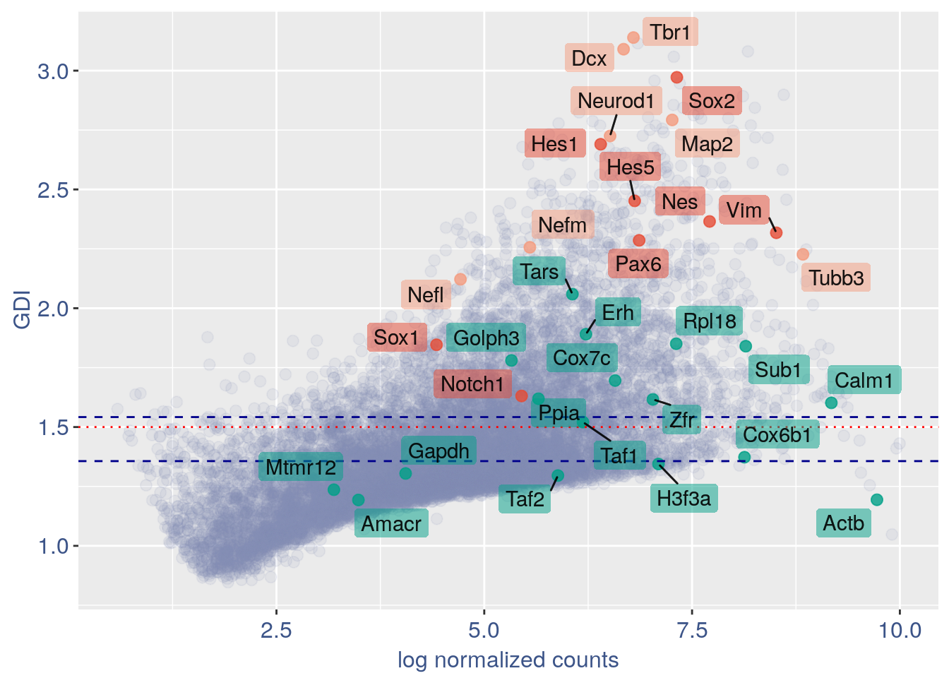
3.3 Heatmaps with cleaning
For the Gene Pair Analysis, we can plot an heatmap with the coex values between two genes sets. To do so we need to define, in a list, the different gene sets (list.genes). Then in the function parameter sets we can decide which sets need to be considered (in the example from 1 to 3). In the condition parameter we should insert an array with each file name prefix to be considered (in the example, the file names is “E11_cortex_clean”).
list.genes = list(Ref.col = PNGs, NPGs = NPGs,
Const. = hk)
plot_heatmap(df_genes = list.genes, sets = c(1:3),
conditions = "E11_cortex_clean", dir = "Data/")
#> [1] "plot heatmap"
#> [1] "Loading condition E11_cortex_clean"
#> [1] "Map2" "Tubb3" "Neurod1" "Nefm" "Nefl" "Dcx" "Tbr1"
#> [1] "Get p-values on a set of genes on columns on a set of genes on rows"
#> [1] "Using function S"
#> [1] "function to generate S "
#> [1] "Ref.col"
#> [1] "NPGs"
#> [1] "Const."
#> [1] "min coex: -0.0104931136392143 max coex 0.0140062494584321"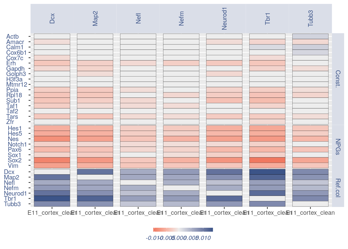 ## Heatmaps without cleaning
list.genes = list(Ref.col = PNGs, NPGs = NPGs,
    Const. = hk)

plot_heatmap(df_genes = list.genes, sets = c(1:3),
    conditions = "E11_cortex", dir = "Data/")
#> [1] "plot heatmap"
#> [1] "Loading condition E11_cortex"
#> [1] "Map2"    "Tubb3"   "Neurod1" "Nefm"    "Nefl"    "Dcx"     "Tbr1"
#> [1] "Get p-values on a set of genes on columns on a set of genes on rows"
#> [1] "Using function S"
#> [1] "function to generate S "
#> [1] "Ref.col"
#> [1] "NPGs"
#> [1] "Const."
#> [1] "min coex: -0.0103430479944429 max coex 0.0138606324053371"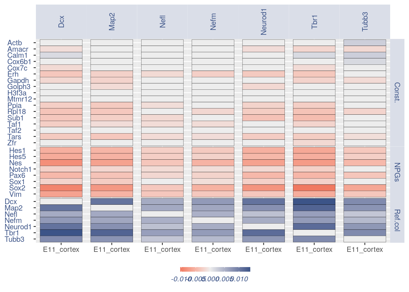
print(sessionInfo())
#> R version 4.0.4 (2021-02-15)
#> Platform: x86_64-pc-linux-gnu (64-bit)
#> Running under: Ubuntu 18.04.5 LTS
#>
#> Matrix products: default
#> BLAS:   /usr/lib/x86_64-linux-gnu/openblas/libblas.so.3
#> LAPACK: /usr/lib/x86_64-linux-gnu/libopenblasp-r0.2.20.so
#>
#> locale:
#>  [1] LC_CTYPE=en_US.UTF-8       LC_NUMERIC=C
#>  [3] LC_TIME=en_US.UTF-8        LC_COLLATE=en_US.UTF-8
#>  [5] LC_MONETARY=en_US.UTF-8    LC_MESSAGES=en_US.UTF-8
#>  [7] LC_PAPER=en_US.UTF-8       LC_NAME=C
#>  [9] LC_ADDRESS=C               LC_TELEPHONE=C
#> [11] LC_MEASUREMENT=en_US.UTF-8 LC_IDENTIFICATION=C
#>
#> attached base packages:
#> [1] stats     graphics  grDevices utils     datasets  methods   base
#>
#> other attached packages:
#> [1] ggrepel_0.9.1     ggplot2_3.3.3     Matrix_1.3-2      data.table_1.14.0
#> [5] COTAN_0.1.0
#>
#> loaded via a namespace (and not attached):
#>  [1] sass_0.3.1           tidyr_1.1.2          jsonlite_1.7.2
#>  [4] R.utils_2.10.1       bslib_0.2.4          assertthat_0.2.1
#>  [7] highr_0.8            stats4_4.0.4         yaml_2.2.1
#> [10] pillar_1.5.1         lattice_0.20-41      glue_1.4.2
#> [13] reticulate_1.18      digest_0.6.27        RColorBrewer_1.1-2
#> [16] colorspace_2.0-0     cowplot_1.1.1        htmltools_0.5.1.1
#> [19] R.oo_1.24.0          pkgconfig_2.0.3      GetoptLong_1.0.5
#> [22] purrr_0.3.4          scales_1.1.1         tibble_3.1.0
#> [25] generics_0.1.0       farver_2.1.0         IRanges_2.24.1
#> [28] ellipsis_0.3.1       withr_2.4.1          BiocGenerics_0.36.0
#> [31] magrittr_2.0.1       crayon_1.4.0         evaluate_0.14
#> [34] R.methodsS3_1.8.1    fansi_0.4.2          Cairo_1.5-12.2
#> [37] tools_4.0.4          GlobalOptions_0.1.2  formatR_1.8
#> [40] lifecycle_1.0.0      matrixStats_0.58.0   ComplexHeatmap_2.6.2
#> [43] basilisk.utils_1.2.2 stringr_1.4.0        S4Vectors_0.28.1
#> [46] munsell_0.5.0        cluster_2.1.1        compiler_4.0.4
#> [49] jquerylib_0.1.3      rlang_0.4.10         grid_4.0.4
#> [52] rjson_0.2.20         rappdirs_0.3.3       circlize_0.4.12
#> [55] labeling_0.4.2       rmarkdown_2.7        basilisk_1.2.1
#> [58] gtable_0.3.0         DBI_1.1.1            R6_2.5.0
#> [61] knitr_1.31           dplyr_1.0.4          utf8_1.2.1
#> [64] clue_0.3-58          filelock_1.0.2       shape_1.4.5
#> [67] stringi_1.5.3        parallel_4.0.4       Rcpp_1.0.6
#> [70] vctrs_0.3.6          png_0.1-7            tidyselect_1.1.0
#> [73] xfun_0.22