E17.5 cortex
library(COTAN)
library(data.table)
library(Matrix)
library(ggrepel)
#> Loading required package: ggplot2
#library(latex2exp)
mycolours <- c("A" = "#8491B4B2","B"="#E64B35FF")
my_theme = theme(axis.text.x = element_text(size = 14, angle = 0, hjust = .5, vjust = .5, face = "plain", colour ="#3C5488FF" ),
axis.text.y = element_text( size = 14, angle = 0, hjust = 0, vjust = .5, face = "plain", colour ="#3C5488FF"),
axis.title.x = element_text( size = 14, angle = 0, hjust = .5, vjust = 0, face = "plain", colour ="#3C5488FF"),
axis.title.y = element_text( size = 14, angle = 90, hjust = .5, vjust = .5, face = "plain", colour ="#3C5488FF"))data = as.data.frame(fread(paste(data_dir,"GSM2861514_E175_Only_Cortical_Cells_DGE.txt.gz", sep = "/")))
data = as.data.frame(data)
rownames(data) = data$V1
data = data[,2:ncol(data)]
data[1:10,1:10]
#> CGTTTAGTTTAC TCTAGAACAACG ACCTTTGTTCGT TTGTCTTCTTCG TAAAATATCGCC
#> 0610005C13Rik 0 0 0 0 0
#> 0610007N19Rik 0 0 0 0 0
#> 0610007P14Rik 2 1 1 1 0
#> 0610009B22Rik 1 1 0 0 0
#> 0610009D07Rik 2 3 0 3 0
#> 0610009E02Rik 0 0 0 0 0
#> 0610009L18Rik 0 0 0 2 0
#> 0610009O20Rik 0 0 0 0 0
#> 0610010F05Rik 1 2 2 0 1
#> 0610010K14Rik 0 0 0 0 0
#> GTACCCTATTTC GCACATTACCCA CCTCGCGCGGCT TTAATTTTGCCT GTCTTGCGTTTT
#> 0610005C13Rik 0 0 0 0 0
#> 0610007N19Rik 0 0 2 0 0
#> 0610007P14Rik 1 0 0 0 0
#> 0610009B22Rik 0 0 1 1 0
#> 0610009D07Rik 2 1 2 1 5
#> 0610009E02Rik 0 0 0 0 0
#> 0610009L18Rik 0 1 1 2 0
#> 0610009O20Rik 0 0 0 1 0
#> 0610010F05Rik 4 0 1 0 2
#> 0610010K14Rik 0 0 0 0 0Define a directory where the ouput will be stored.
1 Analytical pipeline
Initialize the COTAN object with the row count table and the metadata for the experiment.
obj = new("scCOTAN",raw = data)
obj = initRaw(obj,GEO="GSM2861514" ,sc.method="DropSeq",cond = "mouse cortex E17.5")
#> [1] "Initializing S4 object"
Now we can start the cleaning. Analysis requires and starts from a matrix of raw UMI counts after removing possible cell doublets or multiplets and low quality or dying cells (with too high mtRNA percentage, easily done with Seurat or other tools).
If we do not want to consider the mitochondrial genes we can remove them before starting the analysis.
genes_to_rem = rownames(obj@raw[grep('^mt', rownames(obj@raw)),]) #genes to remove : mithocondrial
obj@raw = obj@raw[!rownames(obj@raw) %in% genes_to_rem,]
cells_to_rem = colnames(obj@raw[which(colSums(obj@raw) == 0)])
obj@raw = obj@raw[,!colnames(obj@raw) %in% cells_to_rem]
We want also to define a prefix to identify the sample.
2 Data cleaning
First, we create the directory to store all information regarding the data cleaning.
if(!file.exists(out_dir)){
  dir.create(file.path(out_dir))
}

if(!file.exists(paste(out_dir,"cleaning", sep = ""))){
  dir.create(file.path(out_dir, "cleaning"))
}
ttm = clean(obj)
#> [1] "Start estimation mu with linear method"
#> [1] 12361 880
#> rowname CCGAGTACGTCC
#> 5083 Hbb-bs 635.916703
#> 5081 Hba-a1 205.857651
#> 5084 Hbb-bt 120.253479
#> 11271 Tuba1a 22.420140
#> 6180 Malat1 18.343751
#> 8461 Ptn 14.267362
#> 4936 Gria2 12.229167
#> 1329 Atrx 10.190973
#> 6820 Mycbp2 8.152778
#> 632 Acin1 6.114584
#> 664 Actb 6.114584
#> 1757 Camk2b 6.114584
#> 1767 Caml 6.114584
#> 5502 Iqsec3 6.114584
#> 8483 Ptprd 6.114584
obj = ttm$object
ttm$pca.cell.2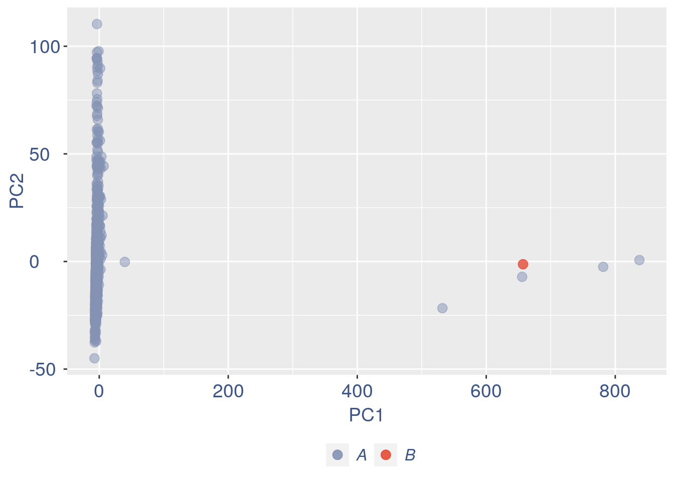
Run this when B cells need to be removed.
pdf(paste(out_dir,"cleaning/",t,"_",n_it,"_plots_before_cells_exlusion.pdf", sep = ""))
ttm$pca.cell.2
ggplot(ttm$D, aes(x=n,y=means)) + geom_point() +
  geom_text_repel(data=subset(ttm$D, n > (max(ttm$D$n)- 15) ), aes(n,means,label=rownames(ttm$D[ttm$D$n > (max(ttm$D$n)- 15),])),
                  nudge_y      = 0.05,
                  nudge_x      = 0.05,
                  direction    = "x",
                  angle        = 90,
                  vjust        = 0,
                  segment.size = 0.2)+
  ggtitle("B cell group genes mean expression")+my_theme +
  theme(plot.title = element_text(color = "#3C5488FF", size = 20, face = "italic",vjust = - 5,hjust = 0.02 ))
#> Warning: ggrepel: 12 unlabeled data points (too many overlaps). Consider
#> increasing max.overlaps
dev.off()
#> png
#>   2

if (length(ttm$cl1) < length(ttm$cl2)) {
  to_rem = ttm$cl1
}else{
  to_rem = ttm$cl2
}
n_it = n_it+1
obj@raw = obj@raw[,!colnames(obj@raw) %in% to_rem]
#obj@raw = obj@raw[rownames(obj@raw) %in% rownames(cells),colnames(obj@raw) %in% colnames(cells)]
gc()
#>            used  (Mb) gc trigger  (Mb) max used  (Mb)
#> Ncells  3728082 199.2    6227150 332.6  6227150 332.6
#> Vcells 75717375 577.7  118003254 900.3 98268863 749.8

ttm = clean(obj)
#> [1] "Start estimation mu with linear method"
#> [1] 12361   879
#>       rowname CGGACATAATGT ACCCGGTCCGAG CACCTGGTCGAC TCGAGTTAAGTC
#> 5083   Hbb-bs  515.0771835  663.4510497  447.1739214   646.150028
#> 5081   Hba-a1  359.0579536  465.9131069  295.5570124   411.900991
#> 5084   Hbb-bt  217.5720219  236.1240715   74.8488538   174.507672
#> 11271  Tuba1a   19.2352475    5.7591237   36.4648262     9.432847
#> 10948  Tmsb4x    4.2744994    1.7277371   21.1112152     1.572141
#> 664      Actb    6.4117492    3.4554742   10.5556076     7.860706
#> 7170     Nnat   12.3960484    6.9109484    0.9596007     3.144282
#> 10944  Tmsb10    4.7019494    0.5759124   12.4748090     4.716424
#> 11279  Tubb2b    3.4195996    2.8795618    9.5960069     3.144282
#> 6395     Meg3    0.4274499    9.7905103    0.0000000     6.288565
#> 11284   Tubb5    5.1293993    1.1518247    6.7172048     3.144282
#> 6180   Malat1    1.2823498    6.3350361    1.9192014     4.716424
#> 1746    Calm1    2.1372497    1.1518247   10.5556076     0.000000
#> 6202    Map1b    2.1372497    1.7277371    6.7172048     3.144282
#> 6065   Lrrc58    2.5646997    1.1518247    4.7980034     4.716424
#ttm = clean.sqrt(obj, cells)
obj = ttm$object

ttm$pca.cell.2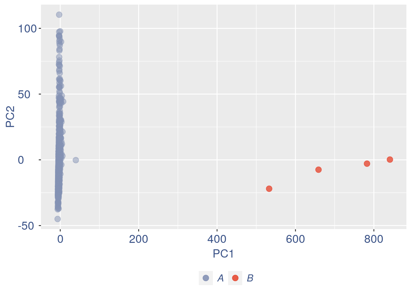
#> Warning: ggrepel: 12 unlabeled data points (too many overlaps). Consider
#> increasing max.overlaps
#> png
#>   2
#>            used  (Mb) gc trigger   (Mb)  max used   (Mb)
#> Ncells  3729046 199.2    6227150  332.6   6227150  332.6
#> Vcells 77512454 591.4  204200820 1558.0 204200082 1558.0
#> [1] "Start estimation mu with linear method"
#> [1] 12350   875
#>       rowname GTGATTGTGTGC CCGGTCAGCAAT TTACTAGCTAAT
#> 6387     Meg3   106.371814   135.402351   134.157606
#> 6173   Malat1    17.406297    37.611764    46.799165
#> 9970   Snhg11    21.274363    56.417646    12.479777
#> 11260  Tuba1a    25.142429     0.000000    18.719666
#> 7162     Nnat     9.670165    30.089411     0.000000
#> 6195    Map1b    15.472264     3.761176     6.239889
#> 9233     Rtn1    11.604198     0.000000    12.479777
#> 11766    Xist     0.000000     0.000000    21.839610
#> 793      Ahi1     1.934033     0.000000    18.719666
#> 9539   Sfrs18     0.000000    11.283529     9.359833
#> 4932    Gria2     5.802099     3.761176     9.359833
#> 11224    Ttc3     5.802099     3.761176     9.359833
#> 7571   Paxbp1     1.934033     3.761176    12.479777
#> 2564    Crmp1     3.868066     7.522353     6.239889
#> 5719    Kif1b     5.802099    11.283529     0.000000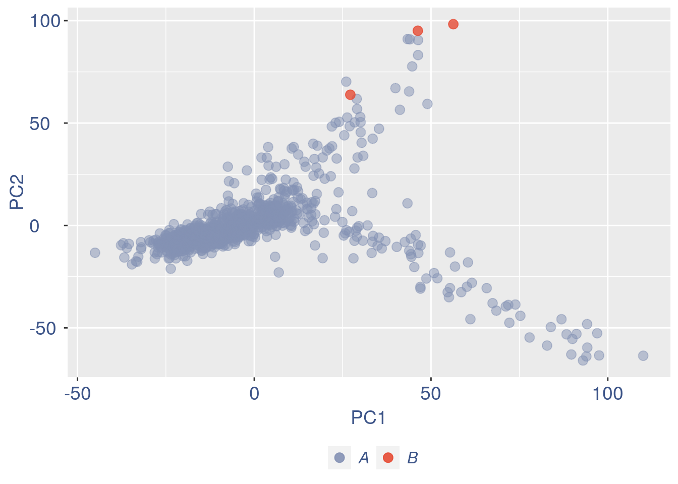
Run this only in the last iteration, instead the previous code, when B cells group has not to be removed.
pdf(paste(out_dir,"cleaning/",t,"_",n_it,"_plots_before_cells_exlusion.pdf", sep = ""))
ttm$pca.cell.2
ggplot(ttm$D, aes(x=n,y=means)) + geom_point() +
  geom_text_repel(data=subset(ttm$D, n > (max(ttm$D$n)- 15) ), aes(n,means,label=rownames(ttm$D[ttm$D$n > (max(ttm$D$n)- 15),])),
                  nudge_y      = 0.05,
                  nudge_x      = 0.05,
                  direction    = "x",
                  angle        = 90,
                  vjust        = 0,
                  segment.size = 0.2)+
  ggtitle(label = "B cell group genes mean expression", subtitle = " - B group NOT removed -")+my_theme +
  theme(plot.title = element_text(color = "#3C5488FF", size = 20, face = "italic",vjust = - 10,hjust = 0.02 ),
        plot.subtitle = element_text(color = "darkred",vjust = - 15,hjust = 0.01 ))
#> Warning: ggrepel: 12 unlabeled data points (too many overlaps). Consider
#> increasing max.overlaps

dev.off()
#> png
#>   2
To color the pca based on nu_j (so the cells’ efficiency).
nu_est = round(obj@nu, digits = 7)

plot.nu <-ggplot(ttm$pca_cells,aes(x=PC1,y=PC2, colour = log(nu_est)))

plot.nu = plot.nu + geom_point(size = 1,alpha= 0.8)+
  scale_color_gradient2(low = "#E64B35B2",mid =  "#4DBBD5B2", high =  "#3C5488B2" ,
                        midpoint = log(mean(nu_est)),name = "ln (nu)")+
  ggtitle("Cells PCA coloured by cells efficiency") +
  my_theme +  theme(plot.title = element_text(color = "#3C5488FF", size = 20),
                    legend.title=element_text(color = "#3C5488FF", size = 14,face = "italic"),
                    legend.text = element_text(color = "#3C5488FF", size = 11),
                    legend.key.width = unit(2, "mm"),
                    legend.position="right")

pdf(paste(out_dir,"cleaning/",t,"_plots_PCA_efficiency_colored.pdf", sep = ""))
plot.nu
dev.off()
#> png
#>   2

plot.nu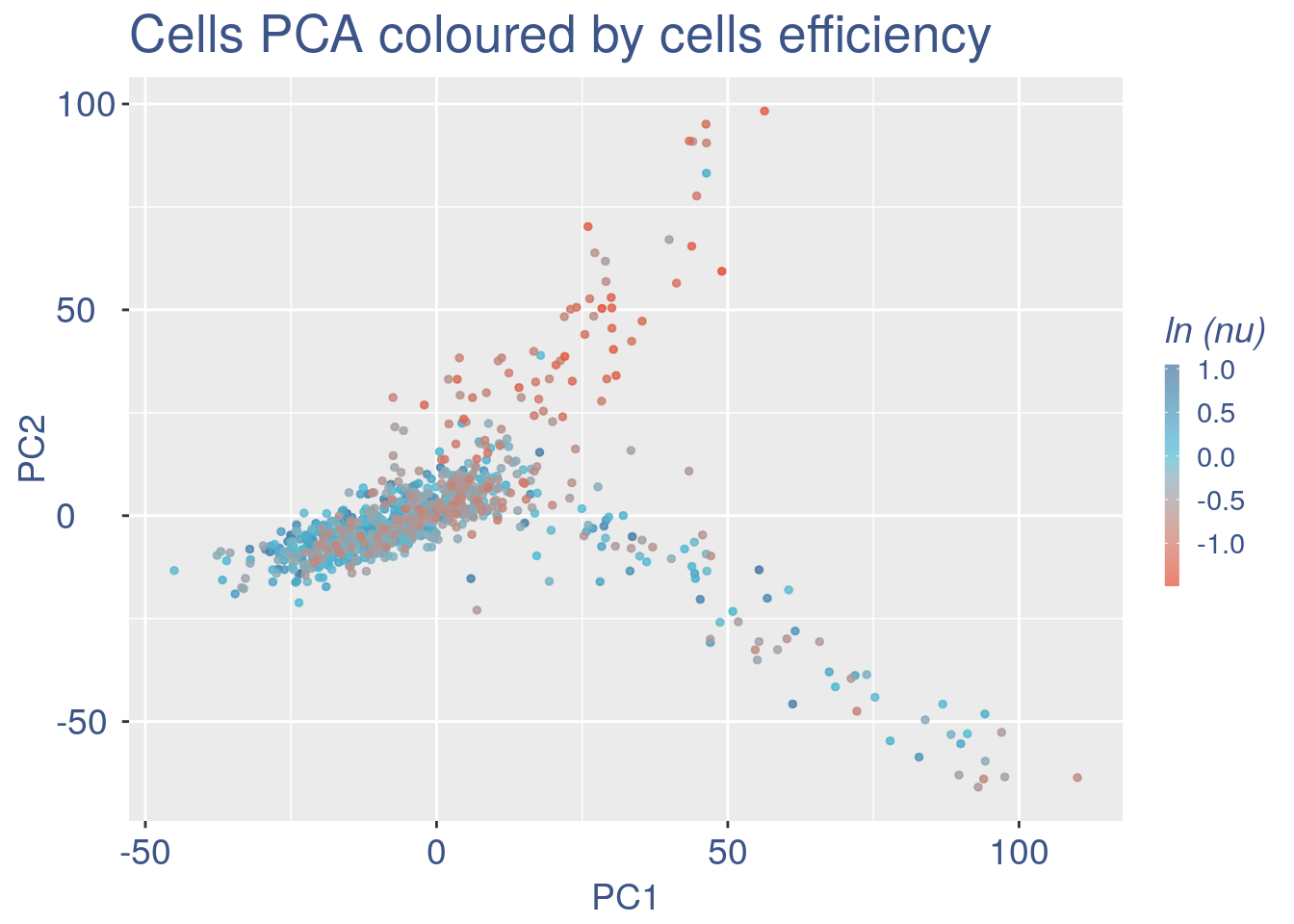
The next part is used to remove the cells with efficiency too low.
nu_df = data.frame("nu"= sort(obj@nu), "n"=c(1:length(obj@nu)))

ggplot(nu_df, aes(x = n, y=nu)) +
    geom_point(colour = "#8491B4B2", size=1)+
    my_theme #+ ylim(0,1) + xlim(0,70)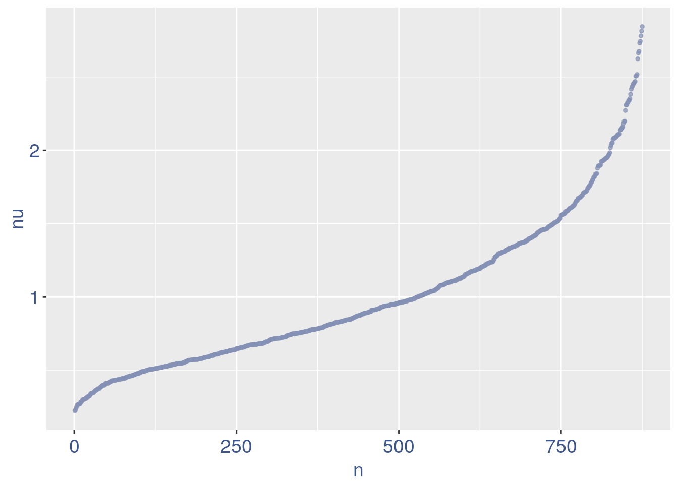
We can zoom on the smallest values and, if we detect a clear elbow, we can decide to remove the cells.
yset = 0.3#threshold to remove low UDE cells
plot.ude <- ggplot(nu_df, aes(x = n, y=nu)) +
    geom_point(colour = "#8491B4B2", size=1) +
    my_theme + ylim(0.,0.7) + xlim(0,200) +
    geom_hline(yintercept=yset, linetype="dashed", color = "darkred") +
    annotate(geom="text", x=500, y=0.5,
             label=paste("to remove cells with nu < ",yset,sep = " "),
             color="darkred", size=4.5)


pdf(paste(out_dir,"cleaning/",t,"_plots_efficiency.pdf", sep = ""))
plot.ude
#> Warning: Removed 675 rows containing missing values (geom_point).
#> Warning: Removed 1 rows containing missing values (geom_text).
dev.off()
#> png
#>   2

plot.ude
#> Warning: Removed 675 rows containing missing values (geom_point).

#> Warning: Removed 1 rows containing missing values (geom_text).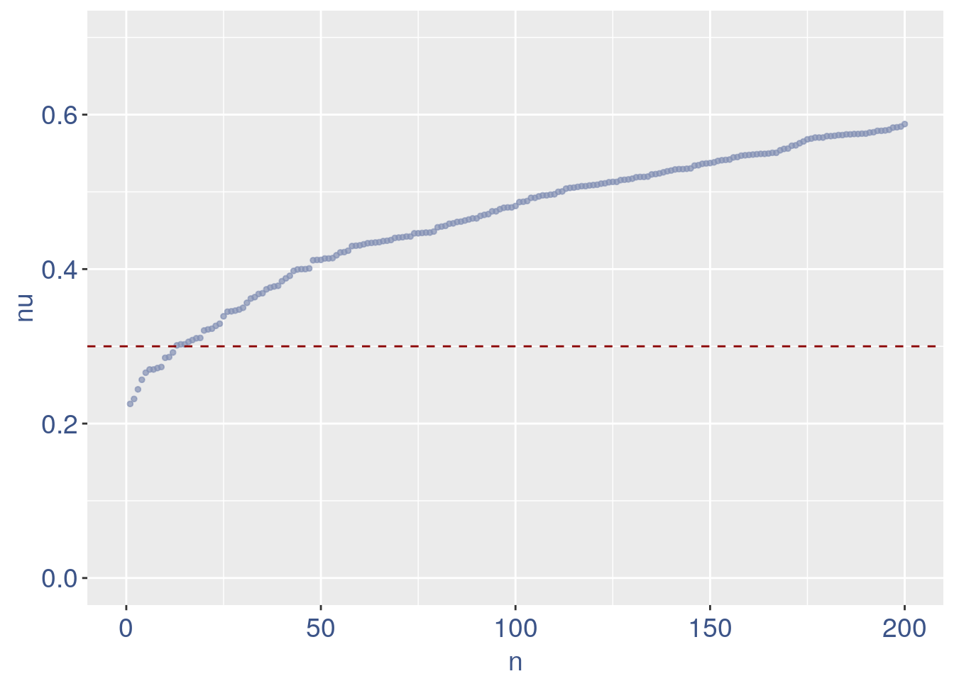
We also save the defined threshold in the metadata and re-run the estimation.
obj@meta[(nrow(obj@meta)+1),1:2] = c("Threshold low UDE cells:",yset)

to_rem = rownames(nu_df[which(nu_df$nu < yset),])

obj@raw = obj@raw[, !colnames(obj@raw) %in% to_rem]
Repeat the estimation after the cells are removed.
ttm = clean(obj)
#> [1] "Start estimation mu with linear method"
#> [1] 12335   863
#>       rowname GTGATTGTGTGC TTACTAGCTAAT
#> 6379     Meg3   107.457036   135.526303
#> 6166   Malat1    17.583879    47.276617
#> 11246  Tuba1a    25.398936    18.910647
#> 9958   Snhg11    21.491407    12.607098
#> 9222     Rtn1    11.722586    12.607098
#> 11752    Xist     0.000000    22.062421
#> 6188    Map1b    15.630114     6.303549
#> 793      Ahi1     1.953764    18.910647
#> 5241    Hook1     3.907529    12.607098
#> 4926    Gria2     5.861293     9.455323
#> 11210    Ttc3     5.861293     9.455323
#> 7562   Paxbp1     1.953764    12.607098
#> 7403    Olfm1     0.000000    12.607098
#> 9461    Sept3     5.861293     6.303549
#> 8473    Ptprs    11.722586     0.000000
obj = ttm$object
ttm$pca.cell.2
Just to check again, we plot the final efficiency coloured PCA.
nu_est = round(obj@nu, digits = 7)
plot.nu <-ggplot(ttm$pca_cells,aes(x=PC1,y=PC2, colour = log(nu_est)))
plot.nu = plot.nu + geom_point(size = 2,alpha= 0.8)+
  scale_color_gradient2(low = "#E64B35B2",mid =  "#4DBBD5B2", high =  "#3C5488B2" ,
                        midpoint = log(mean(nu_est)),name = "ln(nu)")+
  ggtitle("Cells PCA coloured by cells efficiency: last") +
  my_theme +  theme(plot.title = element_text(color = "#3C5488FF", size = 20),
                    legend.title=element_text(color = "#3C5488FF", size = 14,face = "italic"),
                    legend.text = element_text(color = "#3C5488FF", size = 11),
                    legend.key.width = unit(2, "mm"),
                    legend.position="right")

pdf(paste(out_dir,"cleaning/",t,"_plots_PCA_efficiency_colored_FINAL.pdf", sep = ""))
plot.nu
dev.off()
#> png
#>   2

plot.nu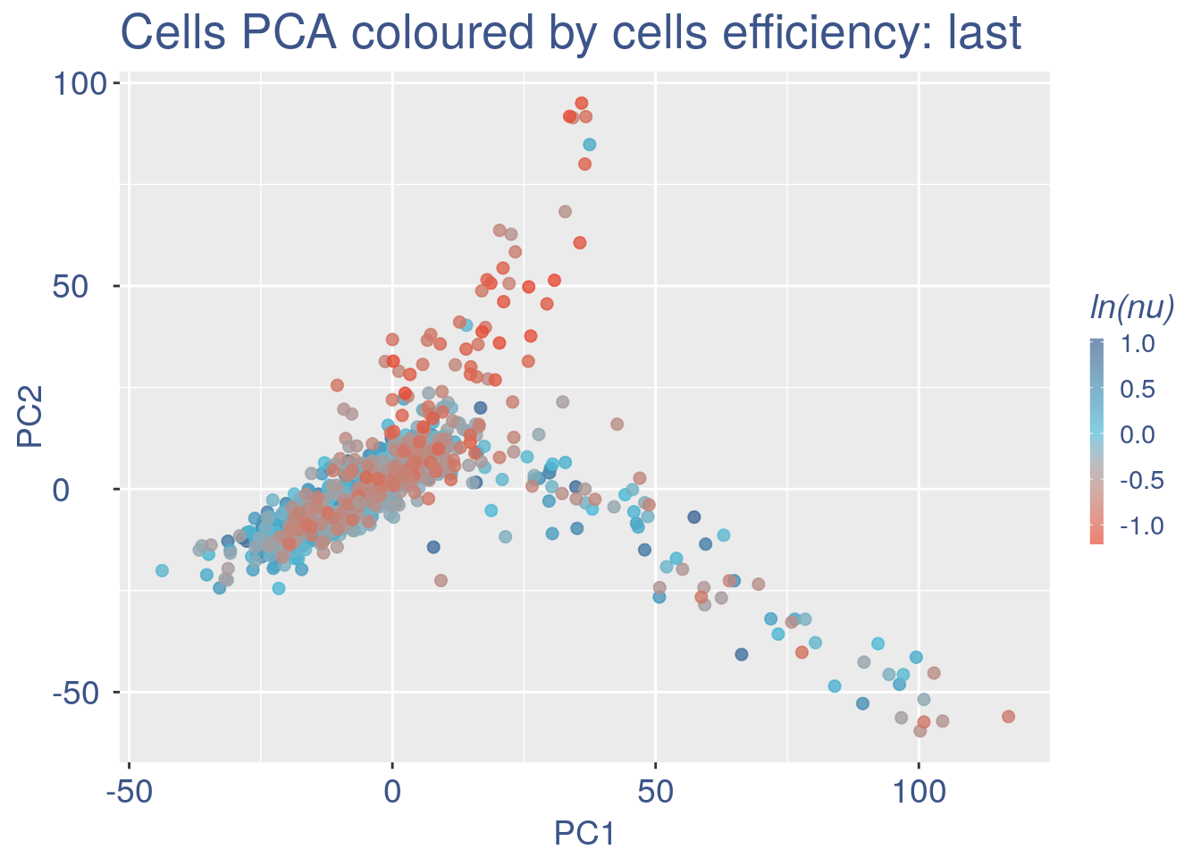
COTAN analysis: in this part all the contingency tables are computed and used to get the statistics (S) To storage efficiency of all the observed tables only the yes_yes is stored. Note that if will be necessary re-computing the yes-yes table, the yes-yes table should be cancelled before running cotan_analysis.
COEX evaluation and storing
3 Analysis of the elaborated data
3.1 GDI
The next function can directly plot the GDI for the dataset with the 1.5 threshold (in red) and the two higher quantiles (in blue).
plot_GDI(obj, cond = "E17.5 cortex")
#> [1] "GDI plot "
#> [1] "function to generate GDI dataframe"
#> [1] "Using S"
#> [1] "function to generate S "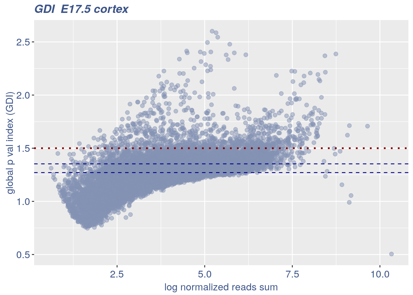
If a more complex plot is needed, or if we want to analyse mor in detail the GDI data, we can get direcly the GDI data frame.
quant.p = get.GDI(obj)
#> [1] "function to generate GDI dataframe"
#> [1] "Using S"
#> [1] "function to generate S "

head(quant.p)
#>               sum.raw.norm      GDI exp.cells
#> 0610007N19Rik     3.344216 1.609840  2.201622
#> 0610007P14Rik     5.325198 1.380006 19.119351
#> 0610009B22Rik     4.754730 1.293699 11.819235
#> 0610009D07Rik     6.329274 1.354907 43.337196
#> 0610009E02Rik     2.599933 1.007798  1.158749
#> 0610009L18Rik     3.564387 1.342003  3.244496
In the third column of this data frame is reported the percentage of cells expressing the gene.
NPGs=c("Nes","Vim","Sox2","Sox1","Notch1", "Hes1","Hes5","Pax6") #,"Hes3"
PNGs=c("Map2","Tubb3","Neurod1","Nefm","Nefl","Dcx","Tbr1")
hk=c("Calm1","Cox6b1","Ppia","Rpl18","Cox7c","Erh","H3f3a","Taf1","Taf2","Gapdh","Actb","Golph3", "Mtmr12", "Zfr", "Sub1", "Tars", "Amacr")

text.size = 12

quant.p$highlight = with(quant.p, ifelse(rownames(quant.p) %in% NPGs, "NPGs",
                                                 ifelse(rownames(quant.p) %in% hk,"Constitutive" ,
                                                               ifelse(rownames(quant.p) %in% PNGs,"PNGs" , "normal"))))

textdf <- quant.p[rownames(quant.p) %in% c(NPGs,hk,PNGs), ]
mycolours <- c("Constitutive" = "#00A087FF","NPGs"="#E64B35FF","PNGs"="#F39B7FFF","normal" = "#8491B4B2")
f1 = ggplot(subset(quant.p,highlight == "normal" ), aes(x=sum.raw.norm, y=GDI)) +  geom_point(alpha = 0.1, color = "#8491B4B2", size=2.5)
GDI_plot = f1 +  geom_point(data = subset(quant.p,highlight != "normal"  ), aes(x=sum.raw.norm, y=GDI, colour=highlight),size=2.5,alpha = 0.8) +
  geom_hline(yintercept=quantile(quant.p$GDI)[4], linetype="dashed", color = "darkblue") +
  geom_hline(yintercept=quantile(quant.p$GDI)[3], linetype="dashed", color = "darkblue") +
  geom_hline(yintercept=1.5, linetype="dotted", color = "red", size= 0.5) +
  scale_color_manual("Status", values = mycolours)  +
  scale_fill_manual("Status", values = mycolours)  +
  xlab("log normalized counts")+ylab("GDI")+
  geom_label_repel(data =textdf , aes(x=sum.raw.norm, y=GDI, label = rownames(textdf),fill=highlight),
                   label.size = NA,
                   alpha = 0.5,
                   direction ="both",
                   na.rm=TRUE,
                   seed = 1234) +
  geom_label_repel(data =textdf , aes(x=sum.raw.norm, y=GDI, label = rownames(textdf)),
                   label.size = NA,
                   segment.color = 'black',
                   segment.size = 0.5,
                   direction = "both",
                   alpha = 0.8,
                   na.rm=TRUE,
                   fill = NA,
                   seed = 1234) +
  theme(axis.text.x = element_text(size = text.size, angle = 0, hjust = .5, vjust = .5, face = "plain", colour ="#3C5488FF" ),
        axis.text.y = element_text( size = text.size, angle = 0, hjust = 0, vjust = .5, face = "plain", colour ="#3C5488FF"),
        axis.title.x = element_text( size = text.size, angle = 0, hjust = .5, vjust = 0, face = "plain", colour ="#3C5488FF"),
        axis.title.y = element_text( size = text.size, angle = 90, hjust = .5, vjust = .5, face = "plain", colour ="#3C5488FF"),
        legend.title = element_blank(),
        legend.text = element_text(color = "#3C5488FF",face ="italic" ),
        legend.position = "bottom")  # titl)
legend <- cowplot::get_legend(GDI_plot)
GDI_plot =GDI_plot + theme(
        legend.position = "none")
GDI_plot
#> Warning: ggrepel: 1 unlabeled data points (too many overlaps). Consider
#> increasing max.overlaps

#> Warning: ggrepel: 1 unlabeled data points (too many overlaps). Consider
#> increasing max.overlaps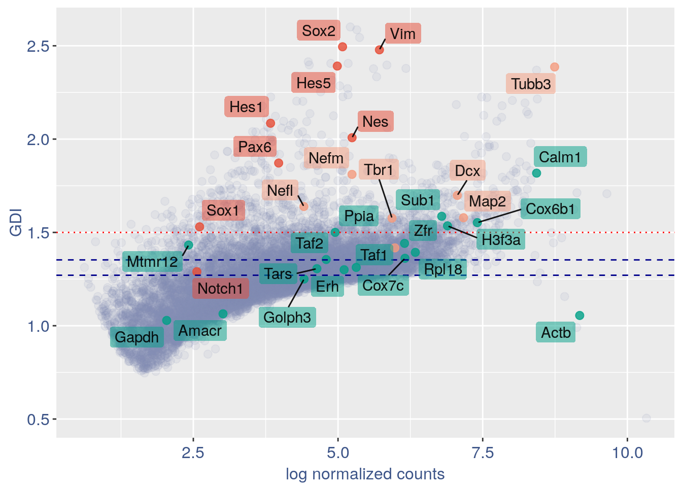
3.2 Heatmaps
For the Gene Pair Analysis, we can plot an heatmap with the coex values between two genes sets. To do so we need to define, in a list, the different gene sets (list.genes). Then in the function parameter sets we can decide which sets need to be considered (in the example from 1 to 3). In the condition parameter we should insert an array with each file name prefix to be considered (in the example, the file names is “E17_cortex_cl2”).
list.genes = list("Ref.col"= PNGs, "NPGs"=NPGs, "Const."=hk )

plot_heatmap(df_genes = list.genes,sets = c(1:3),conditions = "E17_cortex_cl2" ,dir = "Data/")
#> [1] "plot heatmap"
#> [1] "Loading condition E17_cortex_cl2"
#> [1] "Map2"    "Tubb3"   "Neurod1" "Nefm"    "Nefl"    "Dcx"     "Tbr1"
#> [1] "Get p-values on a set of genes on columns on a set of genes on rows"
#> [1] "Using function S"
#> [1] "function to generate S "
#> [1] "Ref.col"
#> [1] "NPGs"
#> [1] "Const."
#> [1] "min coex: -0.0156874873789823 max coex 0.0114906627057202"
print(sessionInfo())
#> R version 4.0.4 (2021-02-15)
#> Platform: x86_64-pc-linux-gnu (64-bit)
#> Running under: Ubuntu 18.04.5 LTS
#>
#> Matrix products: default
#> BLAS:   /usr/lib/x86_64-linux-gnu/openblas/libblas.so.3
#> LAPACK: /usr/lib/x86_64-linux-gnu/libopenblasp-r0.2.20.so
#>
#> locale:
#>  [1] LC_CTYPE=en_US.UTF-8       LC_NUMERIC=C
#>  [3] LC_TIME=en_US.UTF-8        LC_COLLATE=en_US.UTF-8
#>  [5] LC_MONETARY=en_US.UTF-8    LC_MESSAGES=en_US.UTF-8
#>  [7] LC_PAPER=en_US.UTF-8       LC_NAME=C
#>  [9] LC_ADDRESS=C               LC_TELEPHONE=C
#> [11] LC_MEASUREMENT=en_US.UTF-8 LC_IDENTIFICATION=C
#>
#> attached base packages:
#> [1] stats     graphics  grDevices utils     datasets  methods   base
#>
#> other attached packages:
#> [1] ggrepel_0.9.1     ggplot2_3.3.3     Matrix_1.3-2      data.table_1.14.0
#> [5] COTAN_0.1.0
#>
#> loaded via a namespace (and not attached):
#>  [1] Rcpp_1.0.6           lattice_0.20-41      circlize_0.4.12
#>  [4] tidyr_1.1.2          png_0.1-7            assertthat_0.2.1
#>  [7] digest_0.6.27        utf8_1.2.1           R6_2.5.0
#> [10] stats4_4.0.4         evaluate_0.14        highr_0.8
#> [13] pillar_1.5.1         basilisk_1.2.1       GlobalOptions_0.1.2
#> [16] rlang_0.4.10         jquerylib_0.1.3      R.oo_1.24.0
#> [19] R.utils_2.10.1       S4Vectors_0.28.1     GetoptLong_1.0.5
#> [22] reticulate_1.18      rmarkdown_2.7        labeling_0.4.2
#> [25] stringr_1.4.0        munsell_0.5.0        compiler_4.0.4
#> [28] xfun_0.22            pkgconfig_2.0.3      BiocGenerics_0.36.0
#> [31] shape_1.4.5          htmltools_0.5.1.1    tidyselect_1.1.0
#> [34] tibble_3.1.0         IRanges_2.24.1       matrixStats_0.58.0
#> [37] fansi_0.4.2          withr_2.4.1          crayon_1.4.0
#> [40] dplyr_1.0.4          R.methodsS3_1.8.1    rappdirs_0.3.3
#> [43] basilisk.utils_1.2.2 grid_4.0.4           jsonlite_1.7.2
#> [46] gtable_0.3.0         lifecycle_1.0.0      DBI_1.1.1
#> [49] magrittr_2.0.1       scales_1.1.1         stringi_1.5.3
#> [52] farver_2.1.0         bslib_0.2.4          ellipsis_0.3.1
#> [55] filelock_1.0.2       generics_0.1.0       vctrs_0.3.6
#> [58] cowplot_1.1.1        rjson_0.2.20         RColorBrewer_1.1-2
#> [61] tools_4.0.4          Cairo_1.5-12.2       glue_1.4.2
#> [64] purrr_0.3.4          parallel_4.0.4       yaml_2.2.1
#> [67] clue_0.3-58          colorspace_2.0-0     cluster_2.1.1
#> [70] ComplexHeatmap_2.6.2 knitr_1.31           sass_0.3.1