library(ggplot2)
library(tibble)
library(zeallot)
library(COTAN)

options(parallelly.fork.enable = TRUE)

outDir <- "Data/Yuzwa_MouseCortex/"

setLoggingLevel(1)
setLoggingFile(file.path(outDir, "CorticalCells_GSM2861511_E135-analysis.log"))Cortical cells DGE E13.5 Data-set Anaysis
Read the dataset from file:
dataset <- read.csv(file.path("Data/Yuzwa_MouseCortex/", "GSM2861511_E135_Only_Cortical_Cells_DGE.txt.gz"),
                    header = TRUE, sep = "\t", strip.white = TRUE,
                    row.names = 1)
Cleaning
Crate the COTAN object
sampleCondition <- "CorticalCells_GSM2861511_E135"
cc135Obj <- COTAN(raw = dataset)
cc135Obj <- initializeMetaDataset(cc135Obj,
                                  GEO = "GSM2861511_E135",
                                  sequencingMethod = "Drop_seq",
                                  sampleCondition = sampleCondition)
Inspect cells’ sizes
cellSizePlot(cc135Obj)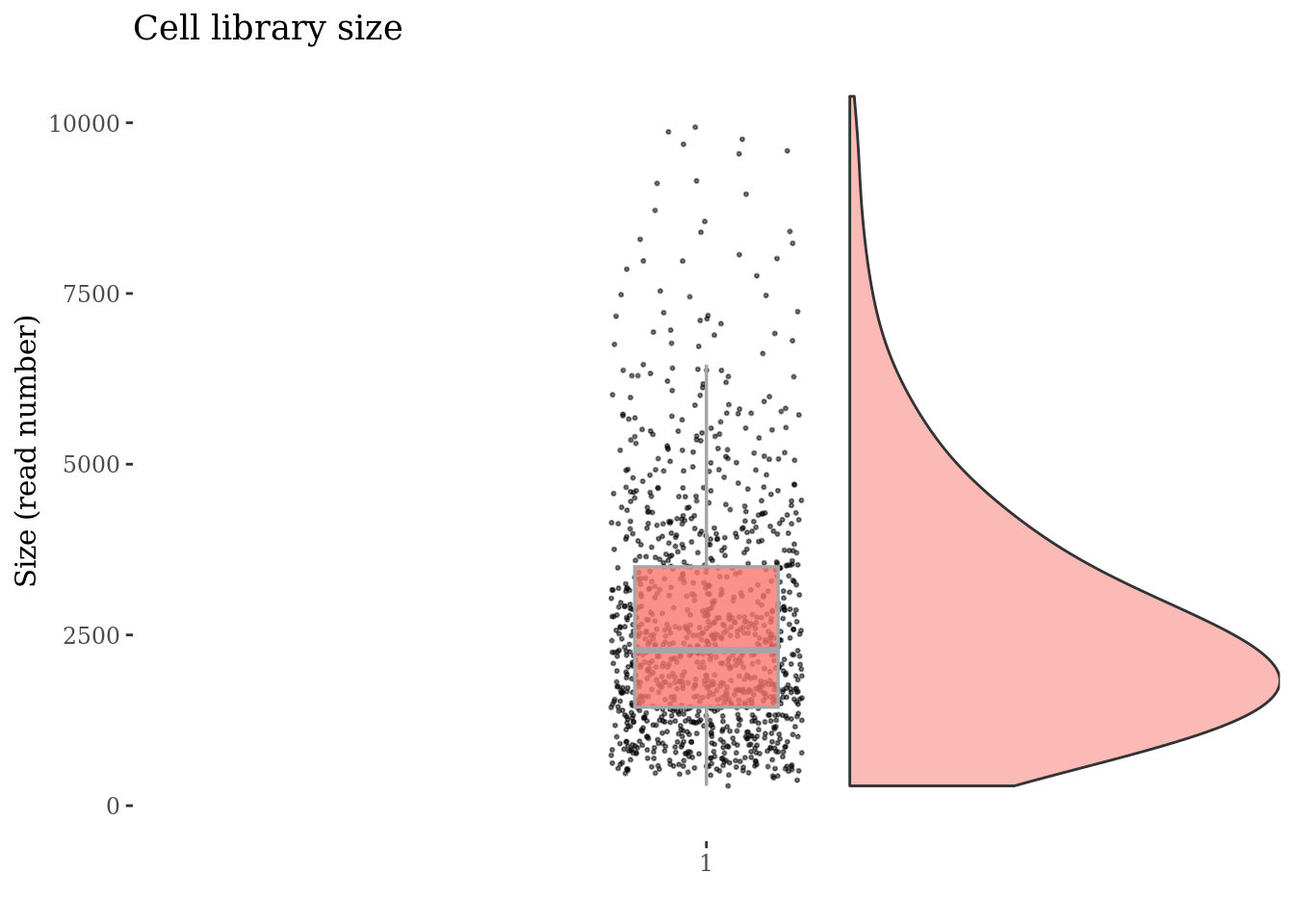
Drop cells with too many ritz reads as they are probably duplets
cellsSizeThr <- 8000
cc135Obj <- addElementToMetaDataset(cc135Obj, "Cells size threshold", cellsSizeThr)

cells_to_rem <- getCells(cc135Obj)[getCellsSize(cc135Obj) > cellsSizeThr]
cc135Obj <- dropGenesCells(cc135Obj, cells = cells_to_rem)

cellSizePlot(cc135Obj)
Inspect the number of expressed genes per cell
genesSizePlot(cc135Obj)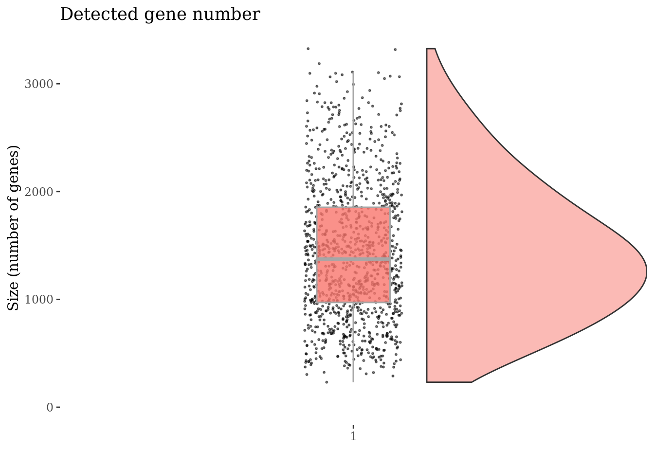
Drop cells with too high genes expession as they are probably duplets
genesSizeThr <- 3300
cc135Obj <- addElementToMetaDataset(cc135Obj, "Num genes threshold", genesSizeThr)

numExprGenes <- getNumExpressedGenes(cc135Obj)
cells_to_rem <- names(numExprGenes)[numExprGenes > genesSizeThr]
cc135Obj <- dropGenesCells(cc135Obj, cells = cells_to_rem)

genesSizePlot(cc135Obj)
Check number of mitocondrial genes expressed in each cell
mitGenesPattern <- "^mt-"
getGenes(cc135Obj)[grep(mitGenesPattern, getGenes(cc135Obj))]
[1] "mt-Co1" "mt-Co3" "mt-Cytb" "mt-Nd1" "mt-Nd2" "mt-Nd4" "mt-Nd5"
[8] "mt-Nd6" "mt-Rnr1" "mt-Rnr2" "mt-Ta" "mt-Tc" "mt-Te" "mt-Tf"
[15] "mt-Ti" "mt-Tl1" "mt-Tl2" "mt-Tm" "mt-Tn" "mt-Tp" "mt-Tq"
[22] "mt-Ts2" "mt-Tt" "mt-Tv" "mt-Tw" c(mitPlot, mitSizes) %<-%
mitochondrialPercentagePlot(cc135Obj, genePrefix = mitGenesPattern)
plot(mitPlot)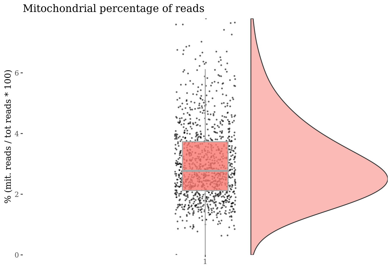
Cells with a too high percentage of mitocondrial genes are likely dead (or at the last problematic) cells. So we drop them!
mitPercThr <- 10.0
cc135Obj <- addElementToMetaDataset(cc135Obj, "Mitoc. perc. threshold", mitPercThr)
cells_to_rem <- rownames(mitSizes)[mitSizes[["mit.percentage"]] > mitPercThr]
cc135Obj <- dropGenesCells(cc135Obj, cells = cells_to_rem)
c(mitPlot, mitSizes) %<-%
  mitochondrialPercentagePlot(cc135Obj, genePrefix = mitGenesPattern)

plot(mitPlot)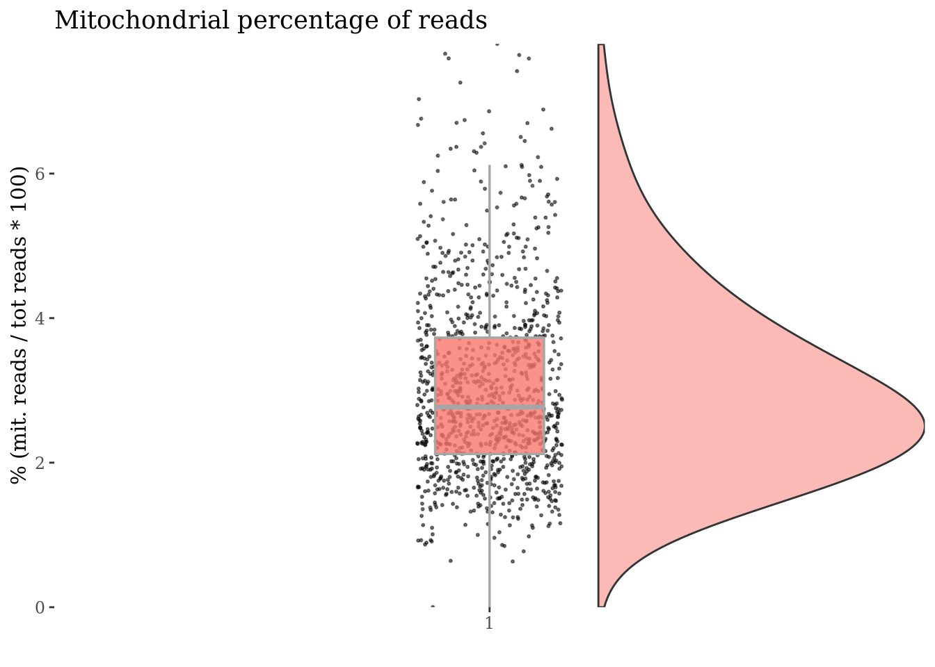
Check no further outliers after all the culling
cellSizePlot(cc135Obj)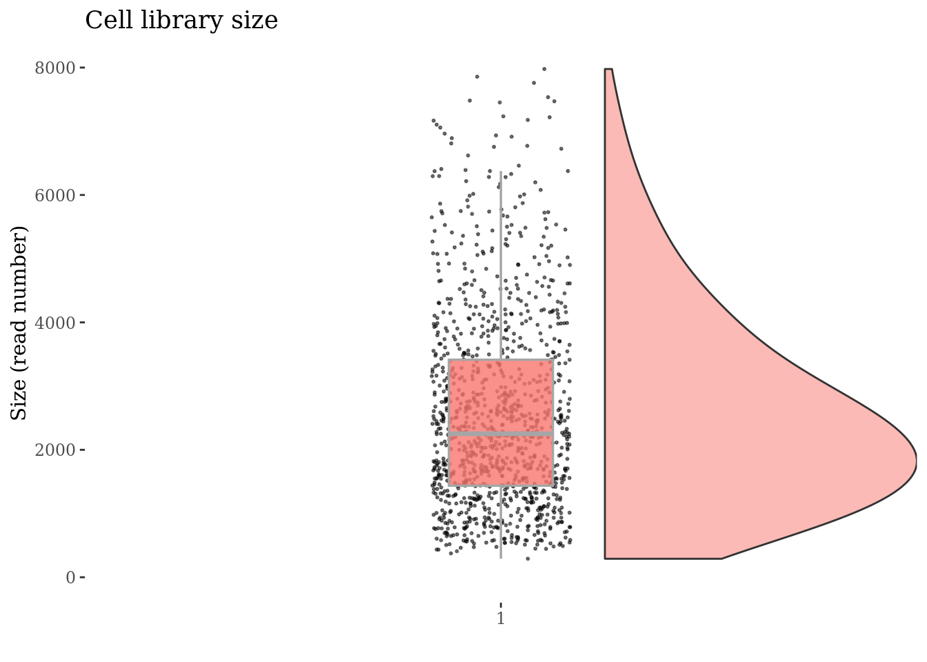
genesSizePlot(cc135Obj)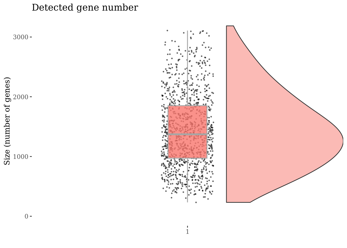
Clean: round 1
cc135Obj <- clean(cc135Obj)

c(pcaCellsPlot, pcaCellsData, genesPlot,
  UDEPlot, nuPlot, zoomedNuPlot) %<-% cleanPlots(cc135Obj)

plot(pcaCellsPlot)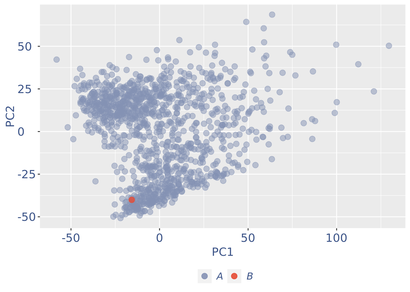
plot(genesPlot)
B group contains high number of hemoglobin genes: so they are not interesting
cells_to_rem <- rownames(pcaCellsData)[pcaCellsData[["groups"]] == "B"]

cc135Obj <- dropGenesCells(cc135Obj, cells = cells_to_rem)
Clean: round 2
cc135Obj <- clean(cc135Obj)

c(pcaCellsPlot, pcaCellsData, genesPlot,
  UDEPlot, nuPlot, zoomedNuPlot) %<-% cleanPlots(cc135Obj)

plot(pcaCellsPlot)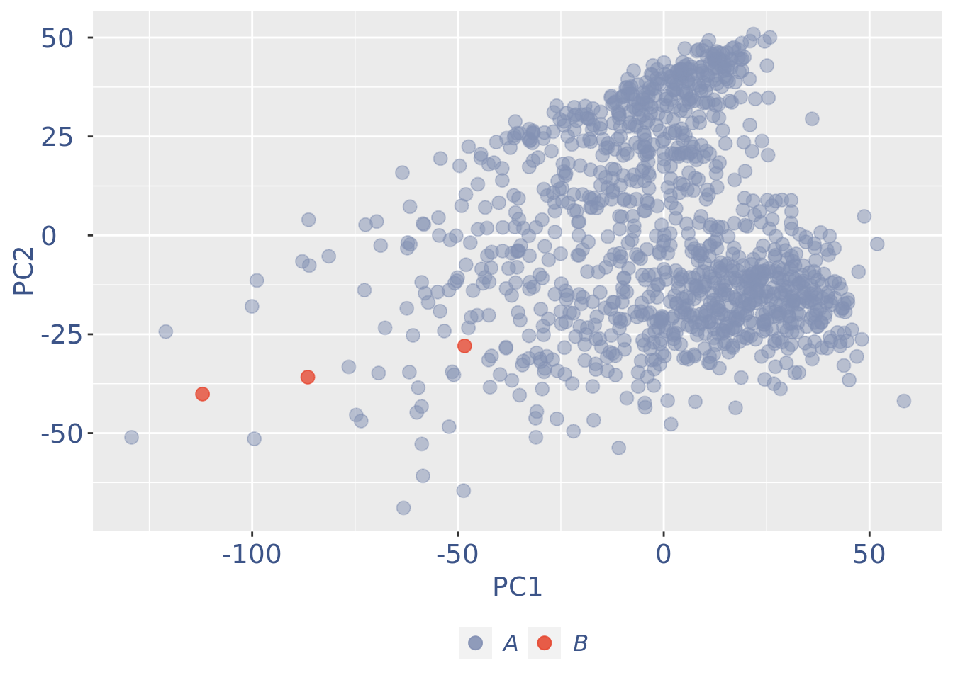
plot(pcaCellsData)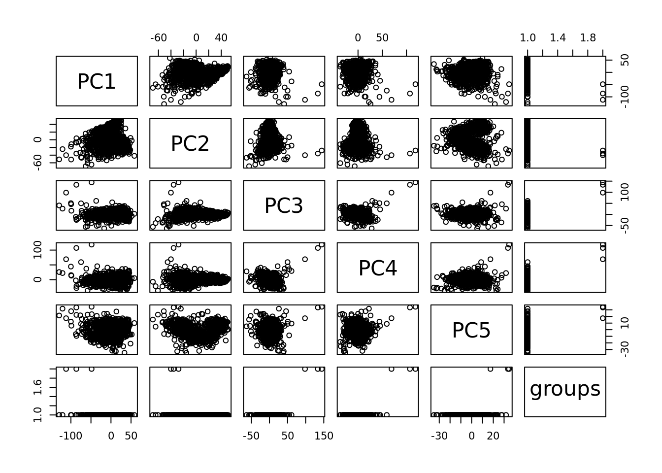
plot(genesPlot)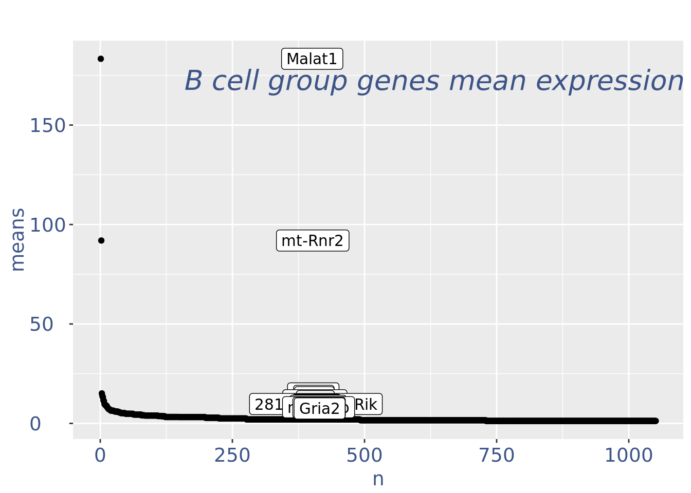
B group contains just 3 cells quite different in the 3rd and 4th components: better to drop them
cells_to_rem <- rownames(pcaCellsData)[pcaCellsData[["groups"]] == "B"]

cc135Obj <- dropGenesCells(cc135Obj, cells = cells_to_rem)
Clean: round 3
cc135Obj <- clean(cc135Obj)

c(pcaCellsPlot, pcaCellsData, genesPlot, UDEPlot, nuPlot, zoomedNuPlot) %<-% cleanPlots(cc135Obj)

plot(pcaCellsPlot)
plot(genesPlot)
cc135Obj <- addElementToMetaDataset(cc135Obj, "Num drop B group", 2)Visualize if all is ok:
plot(UDEPlot)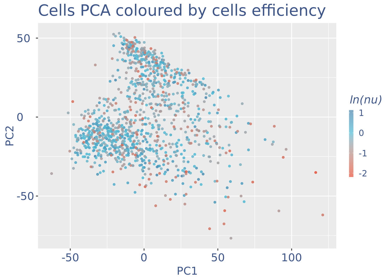
plot(nuPlot)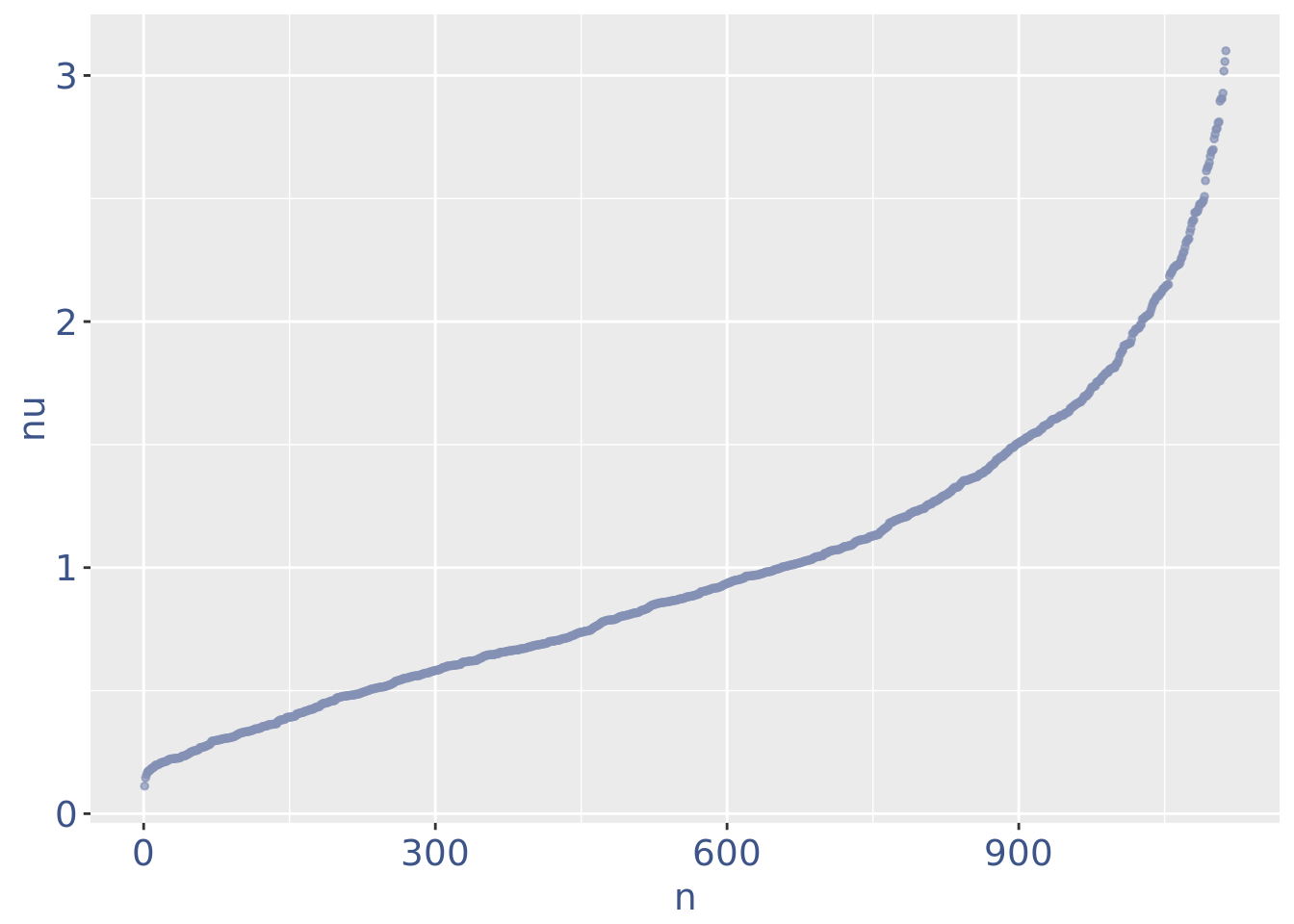
plot(zoomedNuPlot)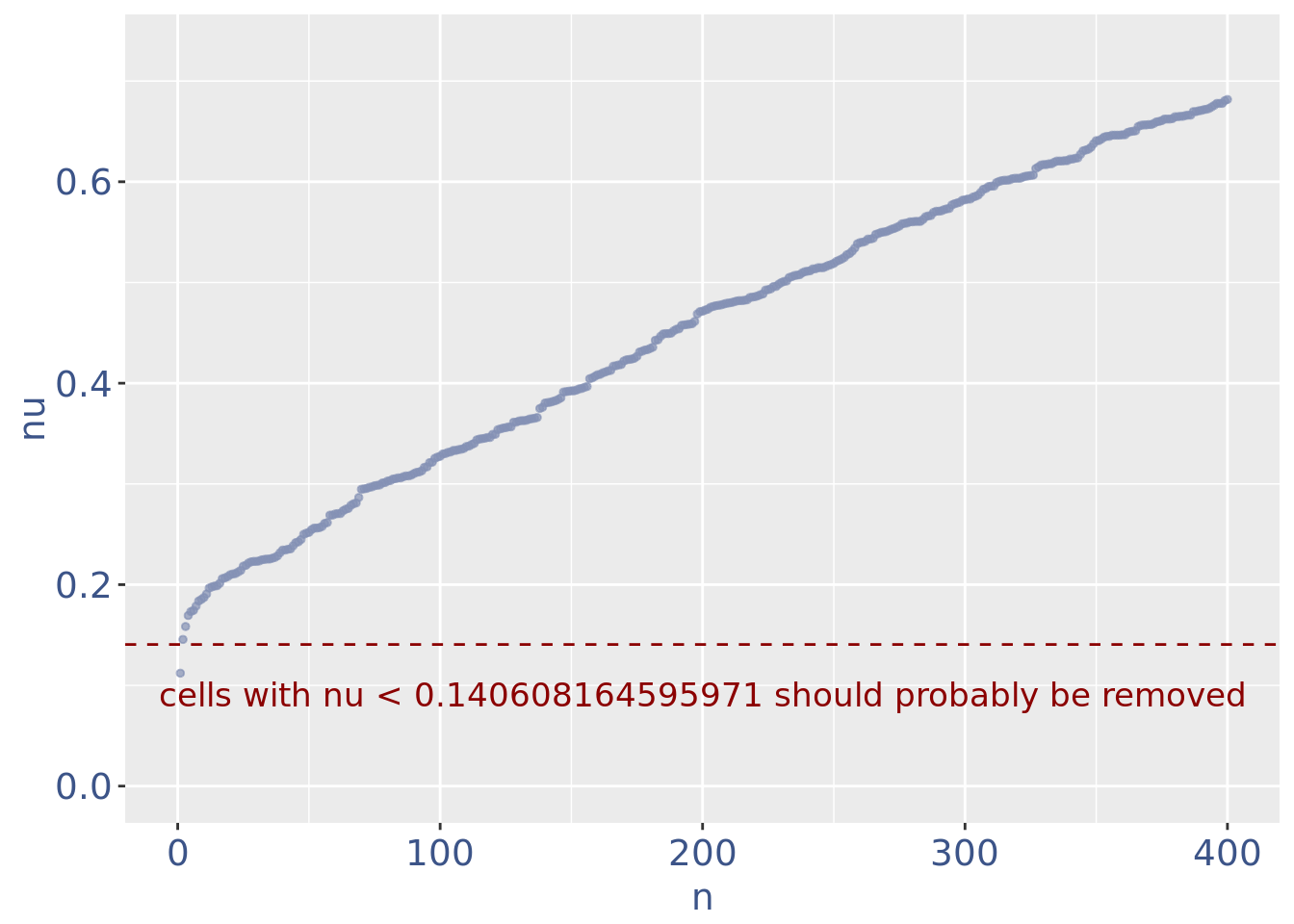
Drop very low UDE cells as they are likely outliers
lowUDEThr <- 0.14 # the threshold to remove low UDE cells

cc135Obj <- addElementToMetaDataset(cc135Obj, "Low UDE threshold", lowUDEThr)

nuDf <- data.frame("nu" = sort(getNu(cc135Obj)), "n" = seq_along(getNu(cc135Obj)))


cells_to_rem <- rownames(nuDf)[nuDf[["nu"]] < lowUDEThr]
cc135Obj <- dropGenesCells(cc135Obj, cells = cells_to_rem)
Final cleaning to check all is OK
cc135Obj <- clean(cc135Obj)

c(pcaCellsPlot, pcaCellsData, genesPlot, UDEPlot, nuPlot, zoomedNuPlot) %<-% cleanPlots(cc135Obj)

plot(pcaCellsPlot)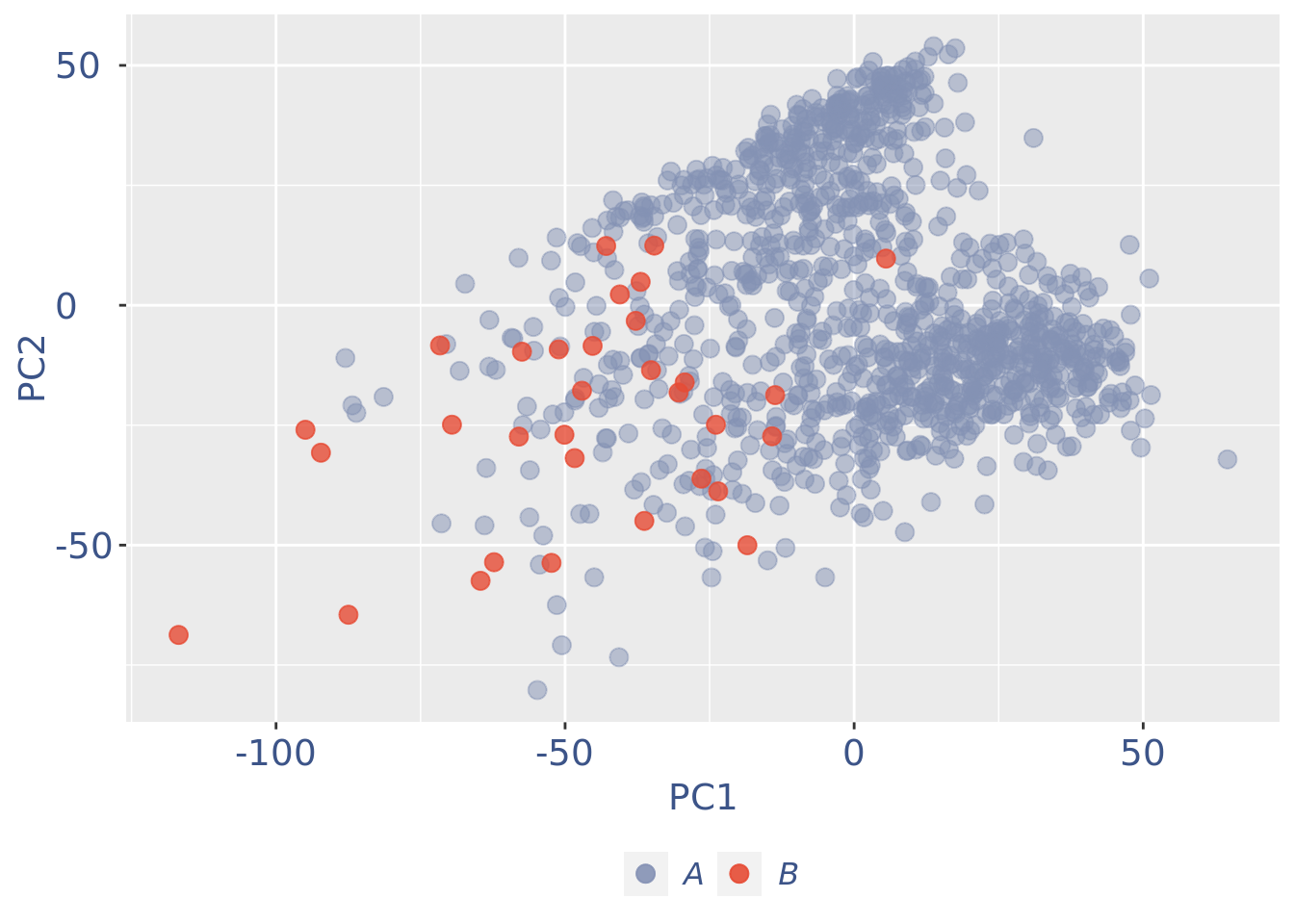
plot(genesPlot)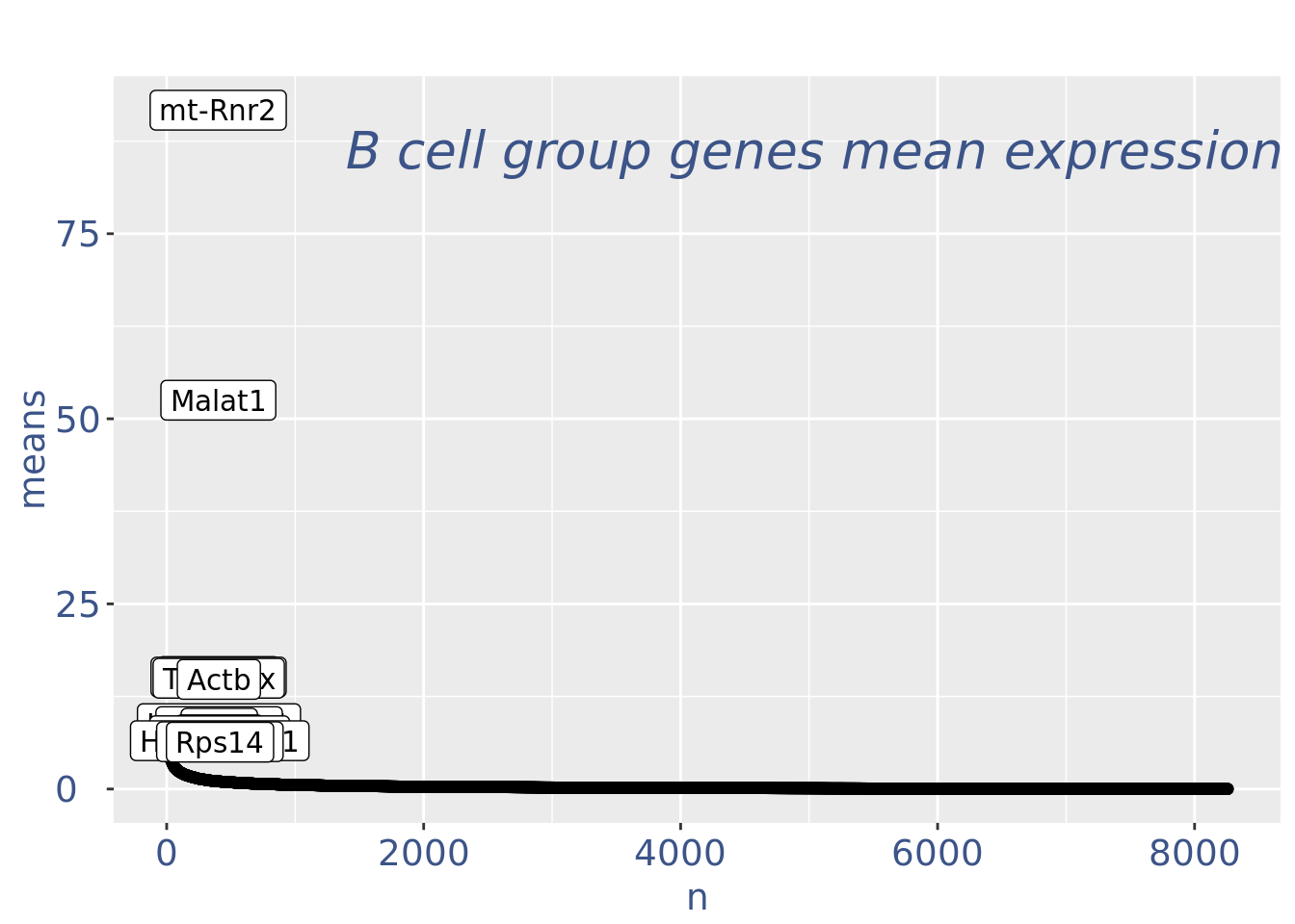
plot(UDEPlot)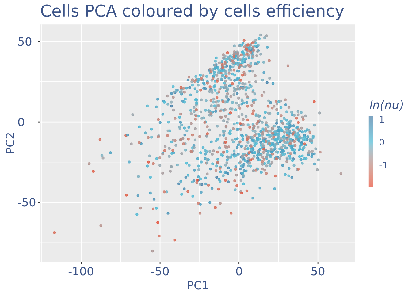
plot(nuPlot)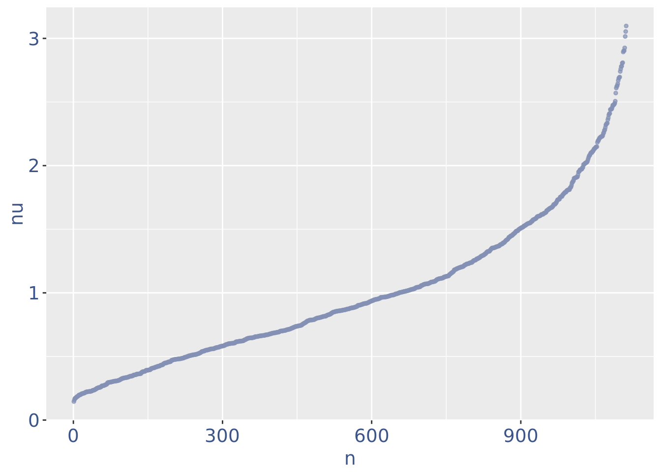
plot(zoomedNuPlot)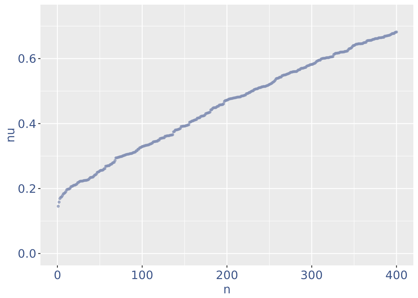
plot(cellSizePlot(cc135Obj))
plot(genesSizePlot(cc135Obj))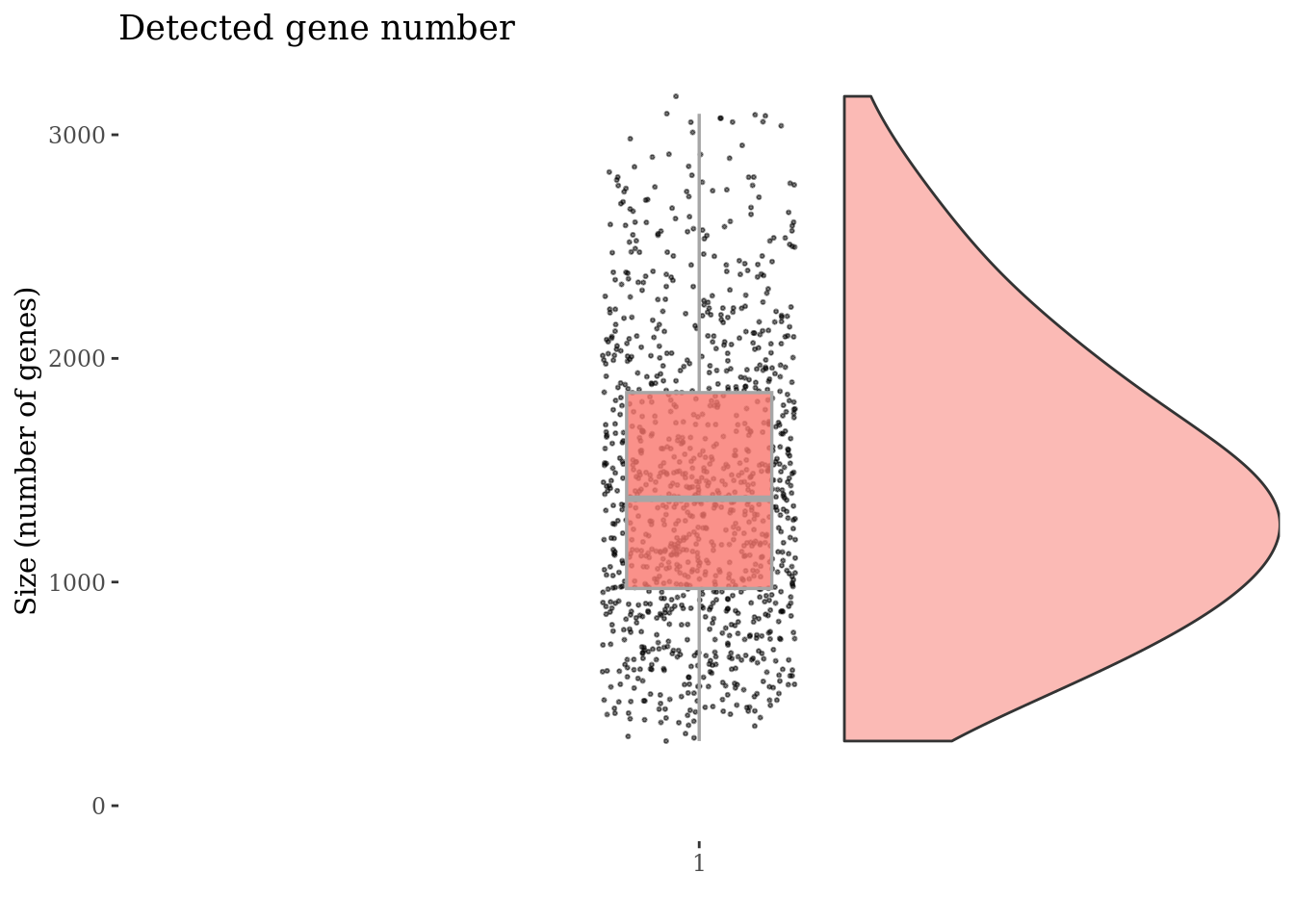
cc135Obj <- proceedToCoex(cc135Obj, calcCoex = TRUE, cores = 12,
                          saveObj = TRUE, outDir = outDir)
Save the COTAN object
saveRDS(cc135Obj, file = file.path(outDir, paste0(sampleCondition, ".cotan.RDS")))GDI
gdiData <- calculateGDI(cc135Obj)

genesToLabel <- head(rownames(gdiData[order(gdiData[["GDI"]],
                                            decreasing = TRUE), ]), n = 10L)

genesToLabel
[1] "Neurod6" "2610017I09Rik" "Nr2e1" "Ina"
[5] "Sox2" "Stmn2" "Mdk" "Mapt"
[9] "Gas1" "2810417H13Rik"gdiPlot <- GDIPlot(cc135Obj, GDIIn = gdiData, GDIThreshold = 1.4,
genes = list("Top 10 GDI genes" = genesToLabel))
plot(gdiPlot)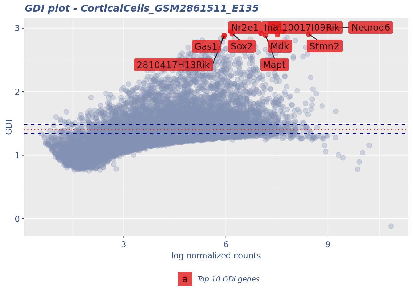
Consistent Transcript Cohorts
c(splitClusters, splitCoexDF) %<-%
  cellsUniformClustering(cc135Obj, GDIThreshold = 1.4, cores = 13,
                         saveObj = TRUE, outDir = outDir)


cc135Obj <- addClusterization(cc135Obj, clName = "split",
                              clusters = splitClusters,
coexDF = splitCoexDF, override = TRUE)table(splitClusters)splitClusters
-1 01 02 03 04 05 06 07 08 09 10 11 12 13 14
6 94 106 47 69 127 92 11 25 12 41 113 59 161 149 saveRDS(cc135Obj, file = file.path(outDir, paste0(sampleCondition, ".cotan.RDS")))c(mergedClusters, mergedCoexDF) %<-%
mergeUniformCellsClusters(cc135Obj, clusters = splitClusters,
GDIThreshold = 1.4, cores = 13,
saveObj = TRUE, outDir = outDir)
cc135Obj <- addClusterization(cc135Obj, clName = "merge",
clusters = mergedClusters,
coexDF = mergedCoexDF,
override = TRUE)table(mergedClusters)mergedClusters
1 2 3 4 5 6 7 8 9
94 153 161 127 113 102 52 161 149 saveRDS(cc135Obj, file = file.path(outDir, paste0(sampleCondition, ".cotan.RDS")))Sys.time()[1] "2025-12-25 16:53:23 CET"sessionInfo()R version 4.5.2 (2025-10-31 ucrt)
Platform: x86_64-w64-mingw32/x64
Running under: Windows 11 x64 (build 26200)
Matrix products: default
LAPACK version 3.12.1
locale:
[1] LC_COLLATE=English_United States.utf8
[2] LC_CTYPE=English_United States.utf8
[3] LC_MONETARY=English_United States.utf8
[4] LC_NUMERIC=C
[5] LC_TIME=English_United States.utf8
time zone: Europe/Rome
tzcode source: internal
attached base packages:
[1] stats graphics grDevices utils datasets methods base
other attached packages:
[1] COTAN_2.11.0 zeallot_0.2.0 tibble_3.3.0 ggplot2_4.0.1
loaded via a namespace (and not attached):
[1] RColorBrewer_1.1-3 jsonlite_2.0.0
[3] shape_1.4.6.1 magrittr_2.0.4
[5] spatstat.utils_3.2-0 farver_2.1.2
[7] rmarkdown_2.30 GlobalOptions_0.1.3
[9] vctrs_0.6.5 ROCR_1.0-11
[11] spatstat.explore_3.6-0 htmltools_0.5.9
[13] S4Arrays_1.10.0 SparseArray_1.10.2
[15] sctransform_0.4.2 parallelly_1.46.0
[17] KernSmooth_2.23-26 htmlwidgets_1.6.4
[19] ica_1.0-3 plyr_1.8.9
[21] plotly_4.11.0 zoo_1.8-14
[23] igraph_2.2.1 mime_0.13
[25] lifecycle_1.0.4 iterators_1.0.14
[27] pkgconfig_2.0.3 rsvd_1.0.5
[29] Matrix_1.7-4 R6_2.6.1
[31] fastmap_1.2.0 MatrixGenerics_1.22.0
[33] fitdistrplus_1.2-4 future_1.68.0
[35] shiny_1.12.1 clue_0.3-66
[37] digest_0.6.39 colorspace_2.1-2
[39] patchwork_1.3.2 S4Vectors_0.48.0
[41] tensor_1.5.1 Seurat_5.3.1
[43] RSpectra_0.16-2 irlba_2.3.5.1
[45] GenomicRanges_1.62.0 beachmat_2.26.0
[47] labeling_0.4.3 progressr_0.18.0
[49] spatstat.sparse_3.1-0 polyclip_1.10-7
[51] httr_1.4.7 abind_1.4-8
[53] compiler_4.5.2 proxy_0.4-28
[55] withr_3.0.2 doParallel_1.0.17
[57] S7_0.2.1 BiocParallel_1.44.0
[59] viridis_0.6.5 fastDummies_1.7.5
[61] dendextend_1.19.1 MASS_7.3-65
[63] DelayedArray_0.36.0 rjson_0.2.23
[65] tools_4.5.2 lmtest_0.9-40
[67] otel_0.2.0 httpuv_1.6.16
[69] future.apply_1.20.1 goftest_1.2-3
[71] glue_1.8.0 nlme_3.1-168
[73] promises_1.5.0 grid_4.5.2
[75] Rtsne_0.17 cluster_2.1.8.1
[77] reshape2_1.4.5 generics_0.1.4
[79] spatstat.data_3.1-9 gtable_0.3.6
[81] tidyr_1.3.1 data.table_1.17.8
[83] BiocSingular_1.26.1 ScaledMatrix_1.18.0
[85] sp_2.2-0 XVector_0.50.0
[87] spatstat.geom_3.6-1 BiocGenerics_0.56.0
[89] RcppAnnoy_0.0.22 ggrepel_0.9.6
[91] RANN_2.6.2 foreach_1.5.2
[93] pillar_1.11.1 stringr_1.6.0
[95] spam_2.11-1 RcppHNSW_0.6.0
[97] later_1.4.4 circlize_0.4.17
[99] splines_4.5.2 dplyr_1.1.4
[101] gghalves_0.1.4 lattice_0.22-7
[103] deldir_2.0-4 survival_3.8-3
[105] tidyselect_1.2.1 SingleCellExperiment_1.32.0
[107] ComplexHeatmap_2.26.0 miniUI_0.1.2
[109] pbapply_1.7-4 knitr_1.50
[111] gridExtra_2.3 Seqinfo_1.0.0
[113] IRanges_2.44.0 SummarizedExperiment_1.40.0
[115] scattermore_1.2 stats4_4.5.2
[117] xfun_0.54 Biobase_2.70.0
[119] matrixStats_1.5.0 stringi_1.8.7
[121] lazyeval_0.2.2 yaml_2.3.12
[123] evaluate_1.0.5 codetools_0.2-20
[125] cli_3.6.5 uwot_0.2.4
[127] RcppParallel_5.1.11-1 xtable_1.8-4
[129] reticulate_1.44.1 Rcpp_1.1.0
[131] spatstat.random_3.4-3 zigg_0.0.2
[133] globals_0.18.0 png_0.1-8
[135] spatstat.univar_3.1-5 parallel_4.5.2
[137] Rfast_2.1.5.2 assertthat_0.2.1
[139] dotCall64_1.2 parallelDist_0.2.7
[141] listenv_0.10.0 ggthemes_5.2.0
[143] viridisLite_0.4.2 scales_1.4.0
[145] ggridges_0.5.7 SeuratObject_5.3.0
[147] purrr_1.2.0 crayon_1.5.3
[149] GetoptLong_1.1.0 rlang_1.1.6
[151] cowplot_1.2.0