library(COTAN)
library(ComplexHeatmap)
library(circlize)
library(dplyr)
library(Hmisc)
library(Seurat)
library(patchwork)
library(Rfast)
library(parallel)
library(doParallel)
library(HiClimR)
library(stringr)
library(fst)

options(parallelly.fork.enable = TRUE)

dataSetFile <- "Data/Yuzwa_MouseCortex/CorticalCells_GSM2861511_E135.cotan.RDS"
name <- str_split(dataSetFile,pattern = "/",simplify = T)[3]
name <- str_remove(name,pattern = ".RDS")

project = "E13.5"

setLoggingLevel(1)
outDir <- "CoexData/"
setLoggingFile(paste0(outDir, "Logs/",name,".log"))

obj <- readRDS(dataSetFile)
file_code = getMetadataElement(obj, datasetTags()[["cond"]])Gene Correlation Analysis E13.5 for Mouse Cortex
Prologue
source("src/Functions.R")To compare the ability of COTAN to asses the real correlation between genes we define some pools of genes:
- Constitutive genes
- Neural progenitor genes
- Pan neuronal genes
- Some layer marker genes
genesList <- list(
  "NPGs"=
    c("Nes", "Vim", "Sox2", "Sox1", "Notch1", "Hes1", "Hes5", "Pax6"),
  "PNGs"=
    c("Map2", "Tubb3", "Neurod1", "Nefm", "Nefl", "Dcx", "Tbr1"),
  "hk"=
    c("Calm1", "Cox6b1", "Ppia", "Rpl18", "Cox7c", "Erh", "H3f3a",
      "Taf1", "Taf2", "Gapdh", "Actb", "Golph3", "Zfr", "Sub1",
      "Tars", "Amacr"),
  "layers" =
    c("Reln","Lhx5","Cux1","Satb2","Tle1","Mef2c","Rorb","Sox5","Bcl11b","Fezf2","Foxp2","Ntf3","Rasgrf2","Pvrl3", "Cux2","Slc17a6", "Sema3c","Thsd7a", "Sulf2", "Kcnk2","Grik3", "Etv1", "Tle4", "Tmem200a", "Glra2", "Etv1","Htr1f", "Sulf1","Rxfp1", "Syt6")
  # From https://www.science.org/doi/10.1126/science.aam8999
)
COTAN
genesFromListExpressed <- unlist(genesList)[unlist(genesList) %in% getGenes(obj)]
int.genes <-getGenes(obj)
coexMat.big <- getGenesCoex(obj)[genesFromListExpressed,genesFromListExpressed]
coexMat <- getGenesCoex(obj)[c(genesList$NPGs,genesList$hk,genesList$PNGs),c(genesList$NPGs,genesList$hk,genesList$PNGs)]
f1 = colorRamp2(seq(-0.5,0.5, length = 3), c("#DC0000B2", "white","#3C5488B2" ))
split.genes <- base::factor(c(rep("NPGs",length(genesList[["NPGs"]])),
rep("HK",length(genesList[["hk"]])),
rep("PNGs",length(genesList[["PNGs"]]))
),
levels = c("NPGs","HK","PNGs"))
lgd = Legend(col_fun = f1, title = "COTAN coex")
htmp <- Heatmap(as.matrix(coexMat),
#width = ncol(coexMat)*unit(2.5, "mm"),
height = nrow(coexMat)*unit(3, "mm"),
cluster_rows = FALSE,
cluster_columns = FALSE,
col = f1,
row_names_side = "left",
row_names_gp = gpar(fontsize = 11),
column_names_gp = gpar(fontsize = 11),
column_split = split.genes,
row_split = split.genes,
cluster_row_slices = FALSE,
cluster_column_slices = FALSE,
heatmap_legend_param = list(
title = "COTAN coex", at = c(-0.5, 0, 0.5),
direction = "horizontal",
labels = c("-0.5", "0", "0.5")
)
)
draw(htmp, heatmap_legend_side="right")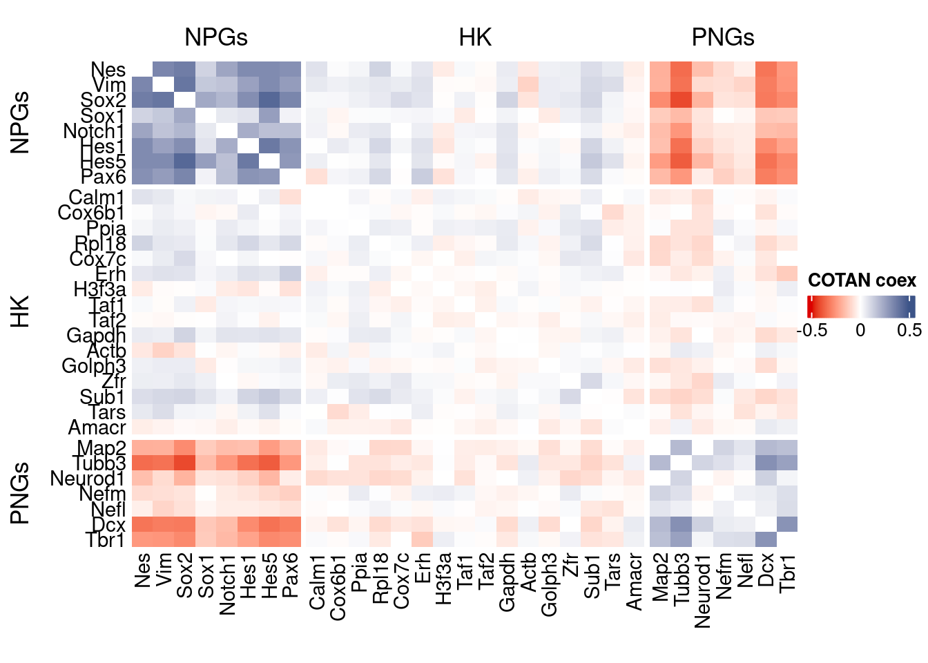
GDI_DF <- calculateGDI(obj)
GDI_DF$geneType <- NA
for (cat in names(genesList)) {
  GDI_DF[rownames(GDI_DF) %in% genesList[[cat]],]$geneType <- cat
}

GDI_DF$GDI_centered <- scale(GDI_DF$GDI,center = T,scale = T)

GDI_DF[genesFromListExpressed,]
sum.raw.norm GDI exp.cells geneType GDI_centered
Nes 6.408692 2.647419 23.1115108 NPGs 4.418329327
Vim 7.312324 2.551967 41.3669065 NPGs 4.083250142
Sox2 6.185654 2.911622 19.1546763 NPGs 5.345792150
Sox1 3.559135 1.880001 2.7877698 NPGs 1.724370053
Notch1 4.800041 2.166044 7.4640288 NPGs 2.728500194
Hes1 4.886836 2.553616 7.9136691 NPGs 4.089038941
Hes5 5.693747 2.751355 11.5107914 NPGs 4.783186933
Pax6 5.993715 2.670699 17.7158273 NPGs 4.500049648
Map2 7.442345 2.359424 59.3525180 PNGs 3.407343330
Tubb3 8.588602 2.719463 79.4964029 PNGs 4.671233319
Neurod1 6.711720 2.015698 26.1690647 PNGs 2.200723866
Nefm 4.837197 1.791972 8.4532374 PNGs 1.415351634
Nefl 3.221387 1.405750 1.8884892 PNGs 0.059550935
Dcx 7.327976 2.605916 53.6870504 PNGs 4.272634438
Tbr1 6.713621 2.557574 37.1402878 PNGs 4.102935005
Calm1 8.848612 1.258354 93.7949640 hk -0.457871717
Cox6b1 7.730664 1.403952 77.6079137 hk 0.053235962
Ppia 5.880634 1.517396 24.1007194 hk 0.451472872
Rpl18 7.242657 1.440153 61.6906475 hk 0.180318242
Cox7c 6.139111 1.409634 31.8345324 hk 0.073183680
Erh 4.868970 1.538559 10.9712230 hk 0.525765263
H3f3a 7.360796 1.375840 68.1654676 hk -0.045447274
Taf1 5.871166 1.296737 20.7733813 hk -0.323130578
Taf2 5.310284 1.282004 13.4892086 hk -0.374852844
Gapdh 3.206206 1.449379 2.3381295 hk 0.212705058
Actb 9.921265 0.894289 99.1906475 hk -1.735893435
Golph3 5.007818 1.281697 10.1618705 hk -0.375928017
Zfr 6.490652 1.446589 35.9712230 hk 0.202909958
Sub1 7.383003 1.618534 62.5899281 hk 0.806510422
Tars 5.450030 1.285601 16.0071942 hk -0.362225062
Amacr 3.191098 1.096773 1.5287770 hk -1.025089118
Reln 3.726806 1.242825 2.1582734 layers -0.512384761
Cux1 5.933575 1.939433 20.8633094 layers 1.933000923
Satb2 5.368174 1.665243 12.6798561 layers 0.970477743
Tle1 4.897234 1.760796 9.8021583 layers 1.305910297
Mef2c 6.152818 2.759922 21.0431655 layers 4.813259827
Rorb 4.875888 1.660140 8.3633094 layers 0.952565229
Sox5 7.276191 2.404274 47.9316547 layers 3.564787044
Bcl11b 7.571149 2.656745 54.0467626 layers 4.451065776
Fezf2 6.718361 2.297884 36.1510791 layers 3.191312576
Foxp2 4.357485 1.350679 4.9460432 layers -0.133772145
Ntf3 2.147161 1.266745 0.8093525 layers -0.428416587
Pvrl3 4.546763 1.600616 6.8345324 layers 0.743609475
Cux2 4.718140 1.538965 6.7446043 layers 0.527188512
Slc17a6 5.699010 1.917841 14.0287770 layers 1.857203373
Sema3c 4.866232 1.435579 7.1942446 layers 0.164262095
Thsd7a 3.836608 1.257654 1.7086331 layers -0.460330847
Sulf2 2.671440 1.498034 1.6187050 layers 0.383504826
Kcnk2 4.495542 1.271818 6.1151079 layers -0.410607221
Grik3 4.020369 1.928627 3.8669065 layers 1.895067663
Etv1 3.735043 1.388003 2.5179856 layers -0.002748532
Tle4 5.288375 1.877388 10.9712230 layers 1.715197034
Tmem200a 2.905427 1.228125 1.5287770 layers -0.563988740
Glra2 4.296262 2.230806 6.3848921 layers 2.955840432
Etv1.1 3.735043 1.388003 2.5179856 layers -0.002748532
Sulf1 1.254408 1.057413 0.3597122 layers -1.163260269
Syt6 4.757203 2.197045 7.5539568 layers 2.837327266GDIPlot(obj,GDIIn = GDI_DF, genes = genesList,GDIThreshold = 1.4)
Seurat correlation
srat<- CreateSeuratObject(counts = getRawData(obj),
                          project = project,
                          min.cells = 3,
                          min.features = 200)
srat[["percent.mt"]] <- PercentageFeatureSet(srat, pattern = "^mt-")
srat <- NormalizeData(srat)
srat <- FindVariableFeatures(srat, selection.method = "vst", nfeatures = 2000)

# plot variable features with and without labels
plot1 <- VariableFeaturePlot(srat)

plot1$data$centered_variance <- scale(plot1$data$variance.standardized,
                                      center = T,scale = F)

write.csv(plot1$data,paste0("CoexData/",
                            "Variance_Seurat_genes",
                            getMetadataElement(obj,
                                               datasetTags()[["cond"]]),".csv"))

LabelPoints(plot = plot1, points = c(genesList$NPGs,genesList$PNGs,genesList$layers), repel = TRUE)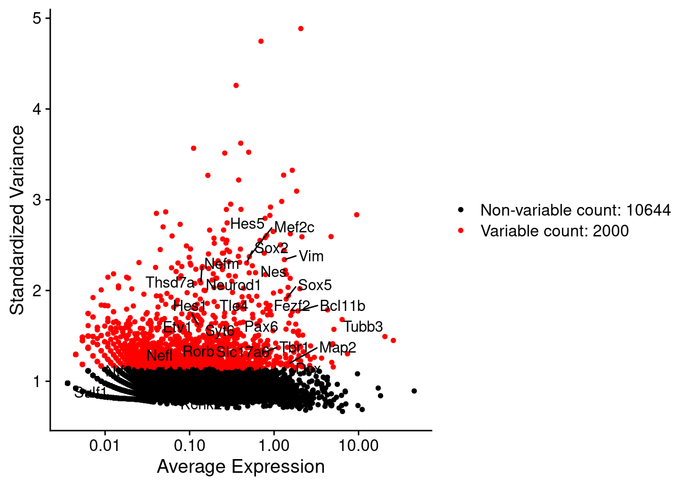
LabelPoints(plot = plot1, points = c(genesList$hk), repel = TRUE)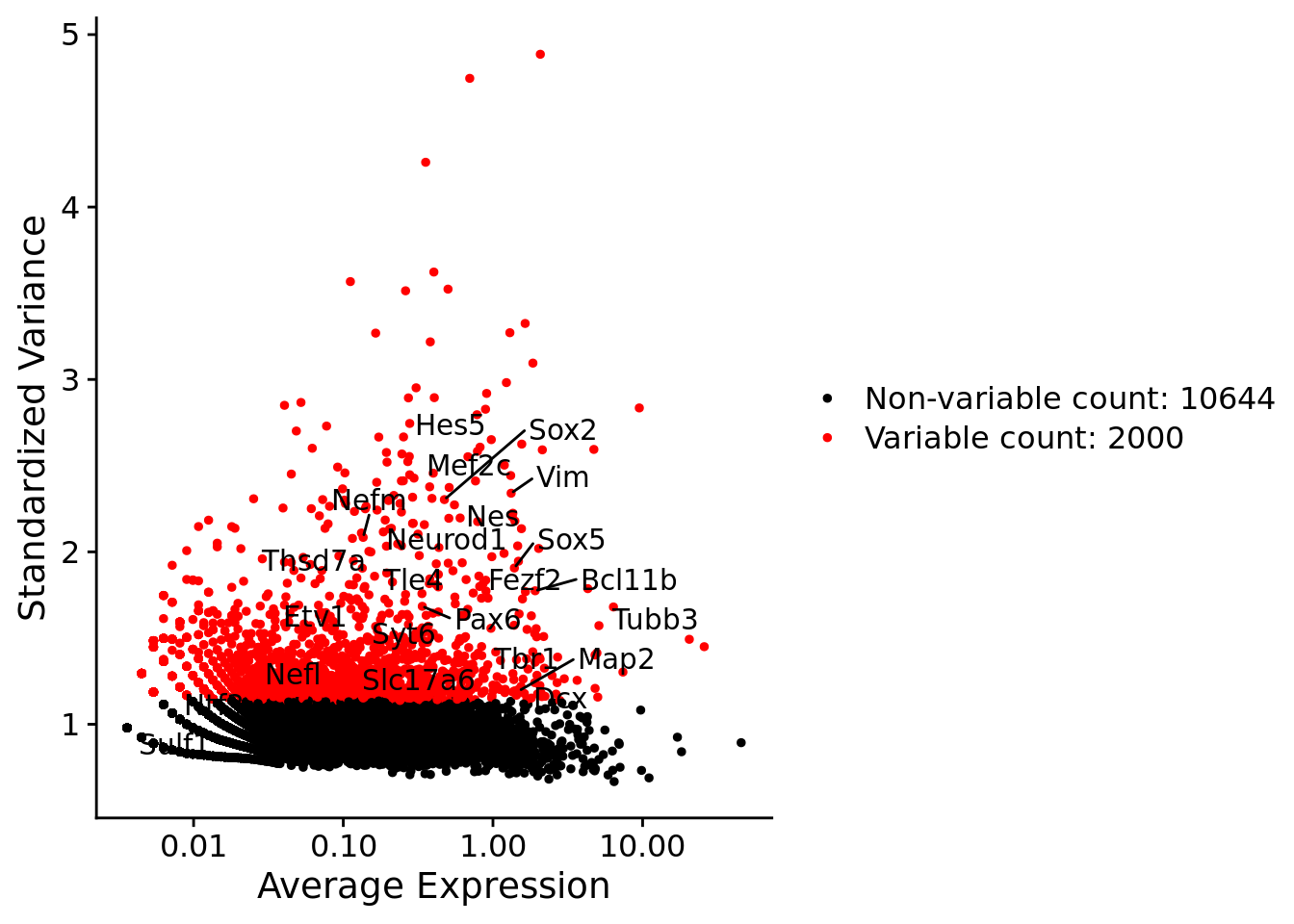
all.genes <- rownames(srat)
srat <- ScaleData(srat, features = all.genes)
seurat.data = GetAssayData(srat[["RNA"]],layer = "data")
corr.pval.list <- correlation_pvalues(data = seurat.data,
genesFromListExpressed,
n.cells = getNumCells(obj))
seurat.data.cor.big <- as.matrix(Matrix::forceSymmetric(corr.pval.list$data.cor, uplo = "U"))
htmp <- correlation_plot(seurat.data.cor.big,
genesList, title="Seurat corr")
p_values.fromSeurat <- corr.pval.list$p_values
seurat.data.cor.big <- corr.pval.list$data.cor
rm(corr.pval.list)
gc() used (Mb) gc trigger (Mb) max used (Mb)
Ncells 10145041 541.9 17741474 947.5 17741474 947.5
Vcells 122134868 931.9 388130163 2961.2 606023191 4623.6draw(htmp, heatmap_legend_side="right")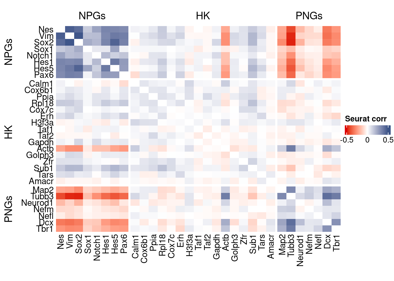
rm(seurat.data.cor.big)
rm(p_values.fromSeurat)
Seurat SC Transform
srat <-  SCTransform(srat,
                     method = "glmGamPoi",
                     vars.to.regress = "percent.mt",
                     verbose = FALSE)

seurat.data <- GetAssayData(srat[["SCT"]],layer = "data")

#Remove genes with all zeros
seurat.data <-seurat.data[rowSums(seurat.data) > 0,]


corr.pval.list <- correlation_pvalues(seurat.data,
                                      genesFromListExpressed,
                                      n.cells = getNumCells(obj))


seurat.data.cor.big <- as.matrix(Matrix::forceSymmetric(corr.pval.list$data.cor, uplo = "U"))

htmp <- correlation_plot(seurat.data.cor.big,
                         genesList, title="Seurat corr SCT")


p_values.fromSeurat <- corr.pval.list$p_values
seurat.data.cor.big <- corr.pval.list$data.cor

rm(corr.pval.list)
gc()
used (Mb) gc trigger (Mb) max used (Mb)
Ncells 10473543 559.4 17741474 947.5 17741474 947.5
Vcells 130551496 996.1 388130163 2961.2 606023191 4623.6draw(htmp, heatmap_legend_side="right")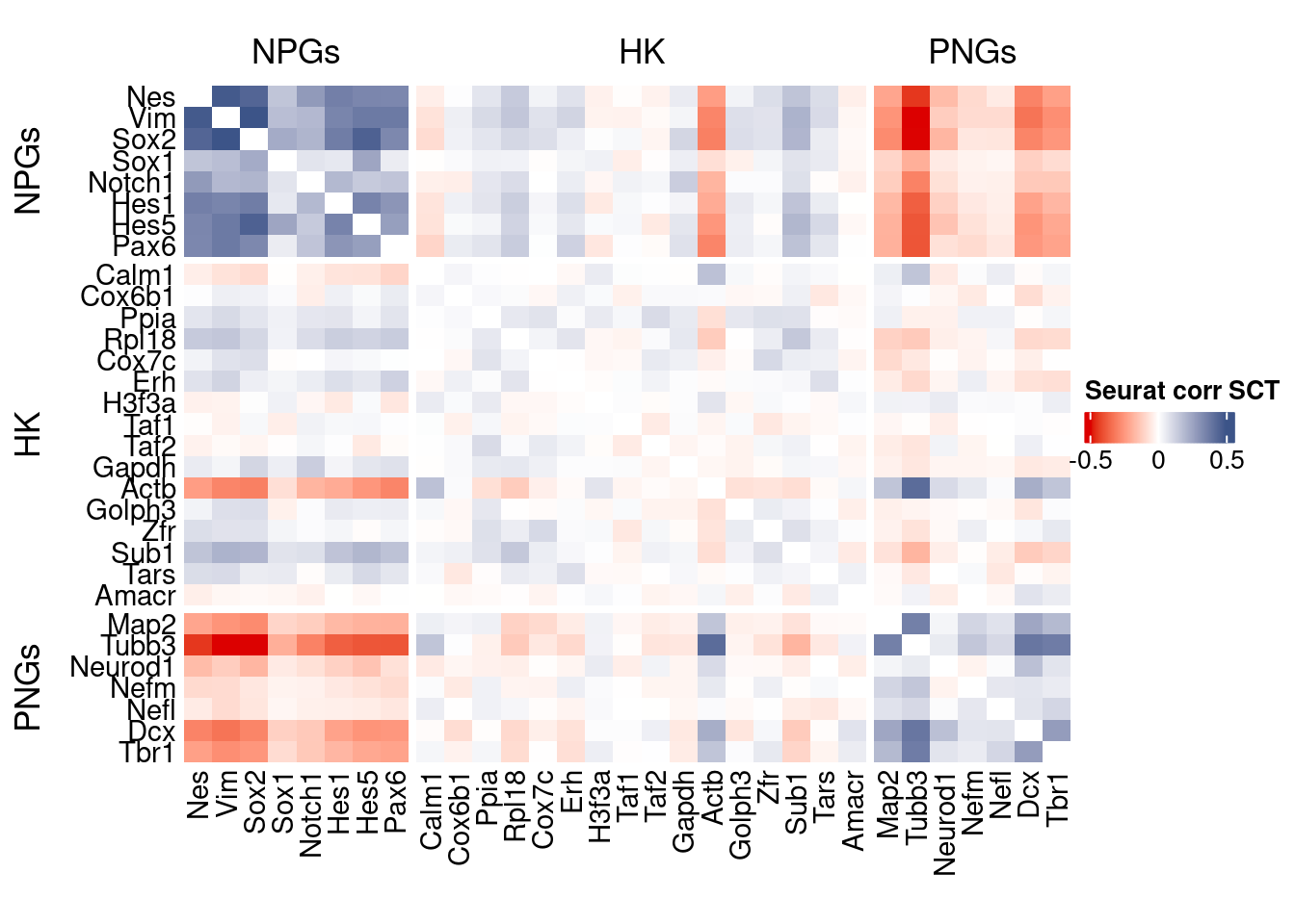
plot1 <- VariableFeaturePlot(srat)

plot1$data$centered_variance <- scale(plot1$data$residual_variance,
center = T,scale = F)write.csv(plot1$data,paste0("CoexData/",
"Variance_SeuratSCT_genes",
getMetadataElement(obj,
datasetTags()[["cond"]]),".csv"))
write_fst(as.data.frame(seurat.data.cor.big),path = paste0("CoexData/SeuratCorrSCT_",file_code,".fst"), compress = 100)
write_fst(as.data.frame(p_values.fromSeurat),path = paste0("CoexData/SeuratPValuesSCT_", file_code,".fst"))
write.csv(as.data.frame(p_values.fromSeurat),paste0("CoexData/SeuratPValuesSCT_", file_code,".csv"))
rm(seurat.data.cor.big)
rm(p_values.fromSeurat)Monocle
library(monocle3)cds <- new_cell_data_set(getRawData(obj),
cell_metadata = getMetadataCells(obj),
gene_metadata = getMetadataGenes(obj)
)
cds <- preprocess_cds(cds, num_dim = 100)
normalized_counts <- normalized_counts(cds)#Remove genes with all zeros
normalized_counts <- normalized_counts[rowSums(normalized_counts) > 0,]
corr.pval.list <- correlation_pvalues(normalized_counts,
genesFromListExpressed,
n.cells = getNumCells(obj))
rm(normalized_counts)
monocle.data.cor.big <- as.matrix(Matrix::forceSymmetric(corr.pval.list$data.cor, uplo = "U"))
htmp <- correlation_plot(data.cor.big = monocle.data.cor.big,
genesList,
title = "Monocle corr")
p_values.from.monocle <- corr.pval.list$p_values
monocle.data.cor.big <- corr.pval.list$data.cor
rm(corr.pval.list)
gc() used (Mb) gc trigger (Mb) max used (Mb)
Ncells 10659808 569.3 17741474 947.5 17741474 947.5
Vcells 132276784 1009.2 388130163 2961.2 606023191 4623.6draw(htmp, heatmap_legend_side="right")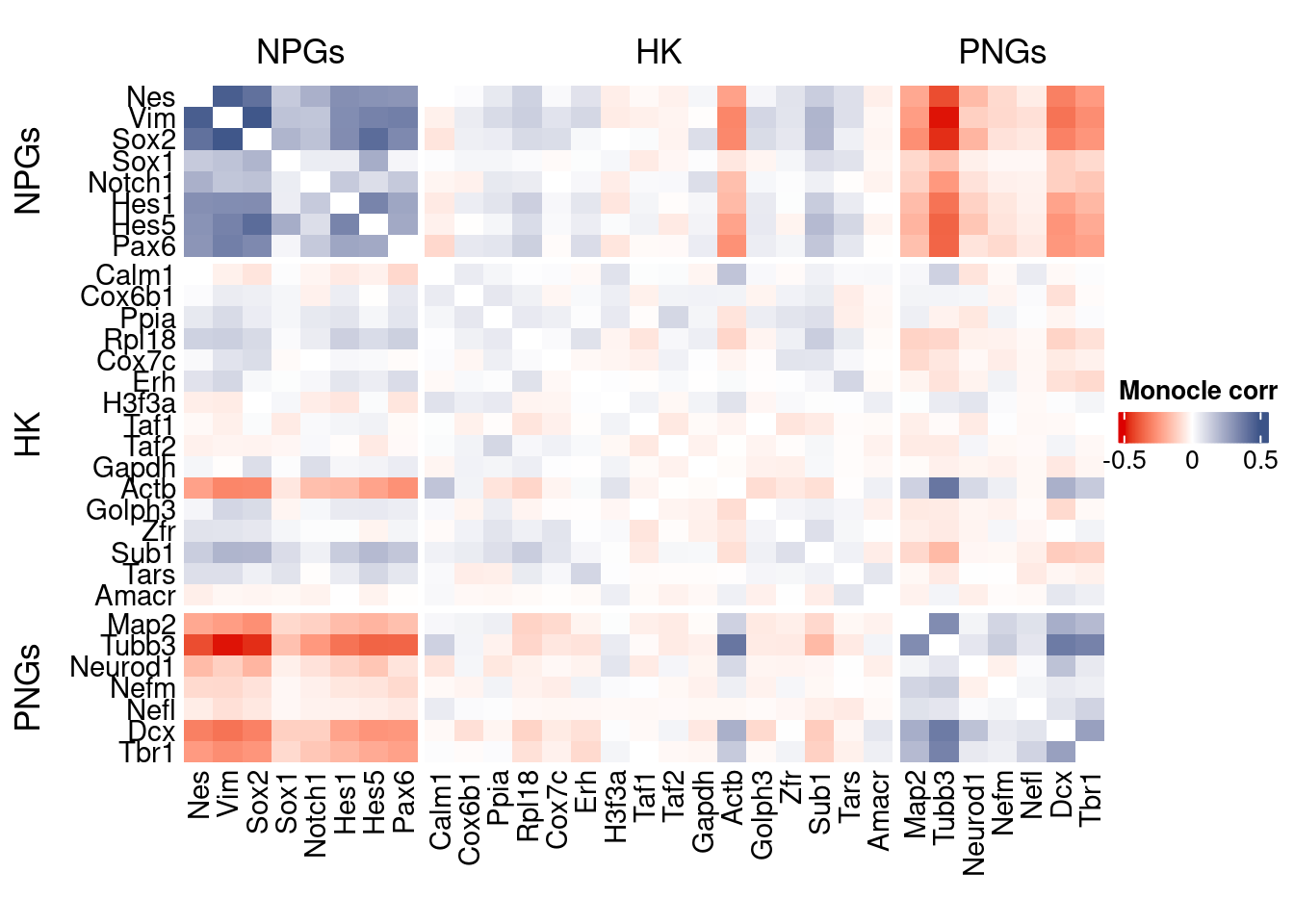
Cs-Core
library(CSCORE)Convert to Seurat obj
sceObj <- convertToSingleCellExperiment(obj)

# Correct: assay=NULL (or omit), data=NULL (since no logcounts)
seuratObj <- as.Seurat(
  x       = sceObj,
  counts  = "counts",
  data    = NULL,
  assay   = NULL,      # IMPORTANT: do NOT set to "RNA" here
  project = "COTAN"
)

# as.Seurat(SCE) creates assay "originalexp" by default; rename it to RNA
seuratObj <- RenameAssays(seuratObj, originalexp = "RNA", verbose = FALSE)
DefaultAssay(seuratObj) <- "RNA"

# Optional: keep COTAN payload
seuratObj@misc$COTAN <- S4Vectors::metadata(sceObj)
Extract CS_CORE corr matrix
#seuratObj@assays$RNA@counts <- ceiling(seuratObj@assays$RNA@counts)
csCoreRes <- CSCORE(seuratObj, genes = genesFromListExpressed)
[INFO] IRLS converged after 3 iterations.
[INFO] Starting WLS for covariance at Wed Jan 21 10:17:47 2026
[INFO] 1 among 57 genes have invalid variance estimates. Their co-expressions with other genes were set to 0.
[INFO] 0.6892% co-expression estimates were greater than 1 and were set to 1.
[INFO] 0.9398% co-expression estimates were smaller than -1 and were set to -1.
[INFO] Finished WLS. Elapsed time: 0.0302 seconds.mat <- as.matrix(csCoreRes$est)
diag(mat) <- 0
split.genes <- base::factor(c(rep("NPGs",sum(genesList[["NPGs"]] %in% genesFromListExpressed)),
rep("HK",sum(genesList[["hk"]] %in% genesFromListExpressed)),
rep("PNGs",sum(genesList[["PNGs"]] %in% genesFromListExpressed))
),
levels = c("NPGs","HK","PNGs"))
f1 = colorRamp2(seq(-0.5,0.5, length = 3), c("#DC0000B2", "white","#3C5488B2" ))
htmp <- Heatmap(as.matrix(mat[c(genesList$NPGs,genesList$hk,genesList$PNGs),c(genesList$NPGs,genesList$hk,genesList$PNGs)]),
#width = ncol(coexMat)*unit(2.5, "mm"),
height = nrow(mat)*unit(3, "mm"),
cluster_rows = FALSE,
cluster_columns = FALSE,
col = f1,
row_names_side = "left",
row_names_gp = gpar(fontsize = 11),
column_names_gp = gpar(fontsize = 11),
column_split = split.genes,
row_split = split.genes,
cluster_row_slices = FALSE,
cluster_column_slices = FALSE,
heatmap_legend_param = list(
title = "CS-CORE", at = c(-0.5, 0, 0.5),
direction = "horizontal",
labels = c("-0.5", "0", "0.5")
)
)
draw(htmp, heatmap_legend_side="right")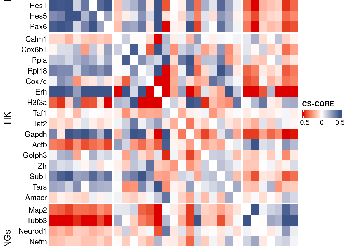
Save CS_CORE matrix
write_fst(as.data.frame(csCoreRes$est), path = paste0("CoexData/CS_CORECorr_", file_code,".fst"),compress = 100)
write_fst(as.data.frame(csCoreRes$p_value), path = paste0("CoexData/CS_COREPValues_", file_code,".fst"),compress = 100)
write.csv(as.data.frame(csCoreRes$p_value), paste0("CoexData/CS_COREPValues_", file_code,".csv"))
Baseline: Spearman on UMI counts
corr.pval.list <- correlation_pvaluesSpearman(data = getRawData(obj),
                                      genesFromListExpressed,
                                      n.cells = getNumCells(obj))

data.cor.big <- as.matrix(Matrix::forceSymmetric(corr.pval.list$data.cor, uplo = "U"))

htmp <- correlation_plot(data.cor.big,
                         genesList, title="UMI baseline S. corr")


p_values.fromSp.C <- corr.pval.list$p_values
data.cor.bigSp.C <- corr.pval.list$data.cor

rm(corr.pval.list)
gc()
used (Mb) gc trigger (Mb) max used (Mb)
Ncells 10668279 569.8 17741474 947.5 17741474 947.5
Vcells 132379412 1010.0 388130163 2961.2 606023191 4623.6draw(htmp, heatmap_legend_side="right")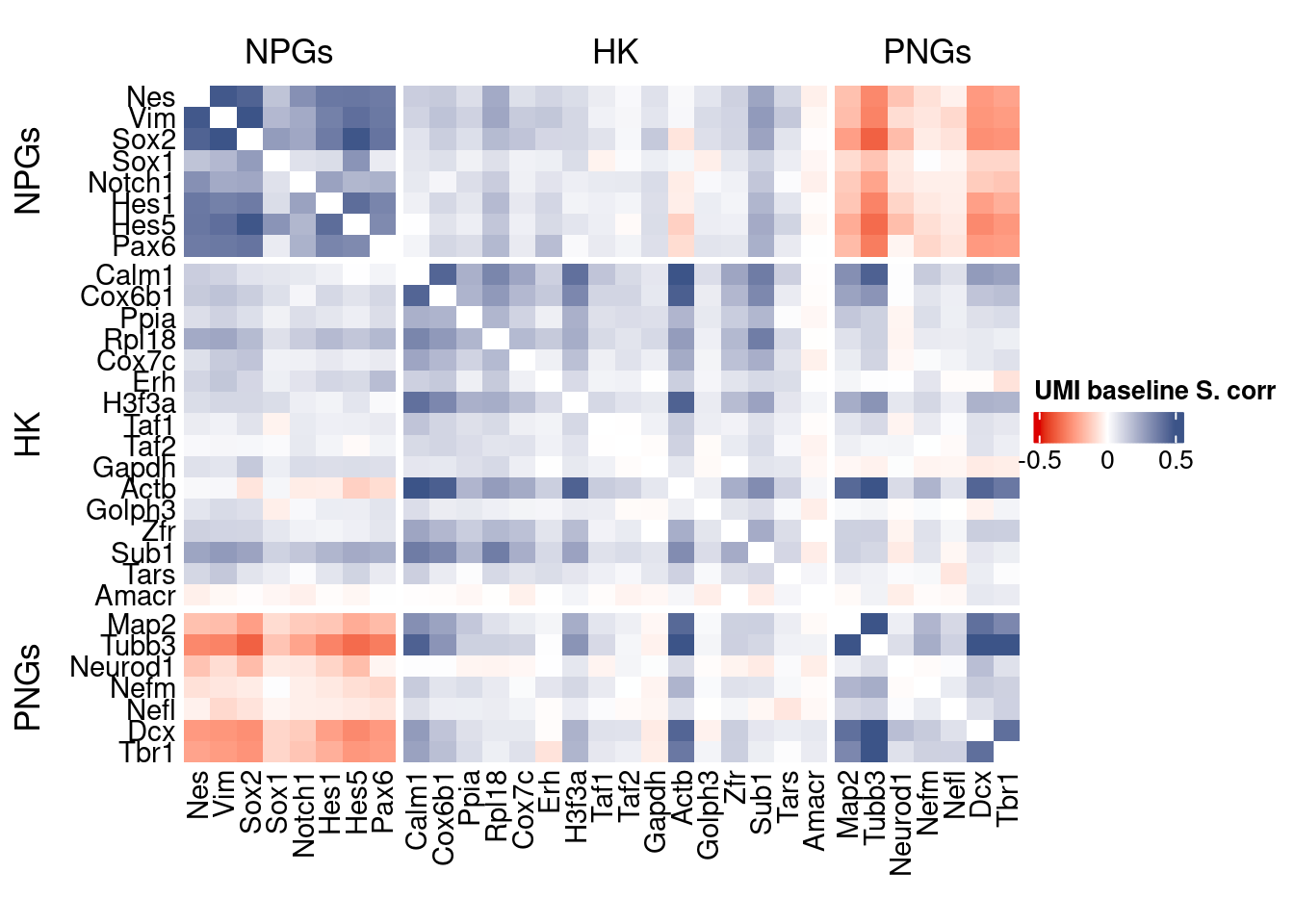
write.csv(as.data.frame(p_values.fromSp.C), paste0("CoexData/BaselineUMISpCorrPValues_", file_code,".csv"))Baseline: Pearson on binarized counts
corr.pval.list <- correlation_pvalues(data = getZeroOneProj(obj),
                                      genesFromListExpressed,
                                      n.cells = getNumCells(obj))

data.cor.big <- as.matrix(Matrix::forceSymmetric(corr.pval.list$data.cor, uplo = "U"))

htmp <- correlation_plot(data.cor.big,
                         genesList, title="Zero-one P. corr")


p_values.fromSp.C <- corr.pval.list$p_values
data.cor.bigSp.C <- corr.pval.list$data.cor

rm(corr.pval.list)
gc()
used (Mb) gc trigger (Mb) max used (Mb)
Ncells 10668313 569.8 17741474 947.5 17741474 947.5
Vcells 132379514 1010.0 388130163 2961.2 606023191 4623.6draw(htmp, heatmap_legend_side="right")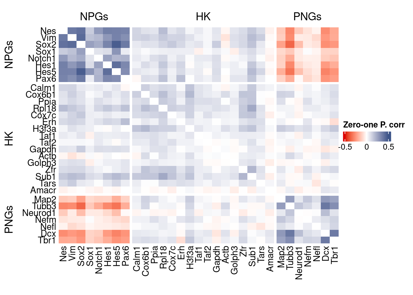
write.csv(as.data.frame(p_values.fromSp.C), paste0("CoexData/ZeroOnePCorrPValues_", file_code,".csv"))Sys.time()[1] "2026-01-21 10:17:51 CET"sessionInfo()R version 4.5.2 (2025-10-31)
Platform: x86_64-pc-linux-gnu
Running under: Ubuntu 22.04.5 LTS
Matrix products: default
BLAS: /usr/lib/x86_64-linux-gnu/blas/libblas.so.3.10.0
LAPACK: /usr/lib/x86_64-linux-gnu/lapack/liblapack.so.3.10.0 LAPACK version 3.10.0
locale:
[1] LC_CTYPE=C.UTF-8 LC_NUMERIC=C LC_TIME=C.UTF-8
[4] LC_COLLATE=C.UTF-8 LC_MONETARY=C.UTF-8 LC_MESSAGES=C.UTF-8
[7] LC_PAPER=C.UTF-8 LC_NAME=C LC_ADDRESS=C
[10] LC_TELEPHONE=C LC_MEASUREMENT=C.UTF-8 LC_IDENTIFICATION=C
time zone: Europe/Rome
tzcode source: system (glibc)
attached base packages:
[1] stats4 parallel grid stats graphics grDevices utils
[8] datasets methods base
other attached packages:
[1] CSCORE_1.0.2 monocle3_1.3.7
[3] SingleCellExperiment_1.32.0 SummarizedExperiment_1.38.1
[5] GenomicRanges_1.62.1 Seqinfo_1.0.0
[7] IRanges_2.44.0 S4Vectors_0.48.0
[9] MatrixGenerics_1.22.0 matrixStats_1.5.0
[11] Biobase_2.70.0 BiocGenerics_0.56.0
[13] generics_0.1.3 fstcore_0.10.0
[15] fst_0.9.8 stringr_1.6.0
[17] HiClimR_2.2.1 doParallel_1.0.17
[19] iterators_1.0.14 foreach_1.5.2
[21] Rfast_2.1.5.1 RcppParallel_5.1.10
[23] zigg_0.0.2 Rcpp_1.1.0
[25] patchwork_1.3.2 Seurat_5.4.0
[27] SeuratObject_5.3.0 sp_2.2-0
[29] Hmisc_5.2-3 dplyr_1.1.4
[31] circlize_0.4.16 ComplexHeatmap_2.26.0
[33] COTAN_2.11.1
loaded via a namespace (and not attached):
[1] RcppAnnoy_0.0.22 splines_4.5.2
[3] later_1.4.2 tibble_3.3.0
[5] polyclip_1.10-7 rpart_4.1.24
[7] fastDummies_1.7.5 lifecycle_1.0.4
[9] Rdpack_2.6.4 globals_0.18.0
[11] lattice_0.22-7 MASS_7.3-65
[13] backports_1.5.0 ggdist_3.3.3
[15] dendextend_1.19.0 magrittr_2.0.4
[17] plotly_4.11.0 rmarkdown_2.29
[19] yaml_2.3.10 httpuv_1.6.16
[21] otel_0.2.0 glmGamPoi_1.20.0
[23] sctransform_0.4.2 spam_2.11-1
[25] spatstat.sparse_3.1-0 reticulate_1.44.1
[27] minqa_1.2.8 cowplot_1.2.0
[29] pbapply_1.7-2 RColorBrewer_1.1-3
[31] abind_1.4-8 Rtsne_0.17
[33] purrr_1.2.0 nnet_7.3-20
[35] GenomeInfoDbData_1.2.14 ggrepel_0.9.6
[37] irlba_2.3.5.1 listenv_0.10.0
[39] spatstat.utils_3.2-1 goftest_1.2-3
[41] RSpectra_0.16-2 spatstat.random_3.4-3
[43] fitdistrplus_1.2-2 parallelly_1.46.0
[45] DelayedMatrixStats_1.30.0 ncdf4_1.24
[47] codetools_0.2-20 DelayedArray_0.36.0
[49] tidyselect_1.2.1 shape_1.4.6.1
[51] UCSC.utils_1.4.0 farver_2.1.2
[53] lme4_1.1-37 ScaledMatrix_1.16.0
[55] viridis_0.6.5 base64enc_0.1-3
[57] spatstat.explore_3.6-0 jsonlite_2.0.0
[59] GetoptLong_1.1.0 Formula_1.2-5
[61] progressr_0.18.0 ggridges_0.5.6
[63] survival_3.8-3 tools_4.5.2
[65] ica_1.0-3 glue_1.8.0
[67] gridExtra_2.3 SparseArray_1.10.8
[69] xfun_0.52 distributional_0.6.0
[71] ggthemes_5.2.0 GenomeInfoDb_1.44.0
[73] withr_3.0.2 fastmap_1.2.0
[75] boot_1.3-32 digest_0.6.37
[77] rsvd_1.0.5 parallelDist_0.2.6
[79] R6_2.6.1 mime_0.13
[81] colorspace_2.1-1 Cairo_1.7-0
[83] scattermore_1.2 tensor_1.5
[85] spatstat.data_3.1-9 tidyr_1.3.1
[87] data.table_1.18.0 httr_1.4.7
[89] htmlwidgets_1.6.4 S4Arrays_1.10.1
[91] uwot_0.2.3 pkgconfig_2.0.3
[93] gtable_0.3.6 lmtest_0.9-40
[95] S7_0.2.1 XVector_0.50.0
[97] htmltools_0.5.8.1 dotCall64_1.2
[99] clue_0.3-66 scales_1.4.0
[101] png_0.1-8 reformulas_0.4.1
[103] spatstat.univar_3.1-6 rstudioapi_0.18.0
[105] knitr_1.50 reshape2_1.4.4
[107] rjson_0.2.23 nloptr_2.2.1
[109] checkmate_2.3.2 nlme_3.1-168
[111] proxy_0.4-29 zoo_1.8-14
[113] GlobalOptions_0.1.2 KernSmooth_2.23-26
[115] miniUI_0.1.2 foreign_0.8-90
[117] pillar_1.11.1 vctrs_0.7.0
[119] RANN_2.6.2 promises_1.5.0
[121] BiocSingular_1.26.1 beachmat_2.26.0
[123] xtable_1.8-4 cluster_2.1.8.1
[125] htmlTable_2.4.3 evaluate_1.0.5
[127] magick_2.9.0 zeallot_0.2.0
[129] cli_3.6.5 compiler_4.5.2
[131] rlang_1.1.7 crayon_1.5.3
[133] future.apply_1.20.0 labeling_0.4.3
[135] plyr_1.8.9 stringi_1.8.7
[137] viridisLite_0.4.2 deldir_2.0-4
[139] BiocParallel_1.44.0 assertthat_0.2.1
[141] lazyeval_0.2.2 spatstat.geom_3.6-1
[143] Matrix_1.7-4 RcppHNSW_0.6.0
[145] sparseMatrixStats_1.20.0 future_1.69.0
[147] ggplot2_4.0.1 shiny_1.12.1
[149] rbibutils_2.3 ROCR_1.0-11
[151] igraph_2.2.1