library(COTAN)
library(ComplexHeatmap)
library(circlize)
library(dplyr)
library(Hmisc)
library(Seurat)
library(patchwork)
library(Rfast)
library(parallel)
library(doParallel)
library(HiClimR)
library(stringr)
library(fst)

options(parallelly.fork.enable = TRUE)

dataSetFile <- "Data/MouseCortexFromLoom/e13.5_ForebrainDorsal.cotan.RDS"

name <- str_split(dataSetFile,pattern = "/",simplify = T)[3]
name <- str_remove(name,pattern = ".RDS")

project = "E13.5"


setLoggingLevel(1)
outDir <- "CoexData/"
setLoggingFile(paste0(outDir, "Logs/",name,".log"))

obj <- readRDS(dataSetFile)
file_code = getMetadataElement(obj, datasetTags()[["cond"]])Gene Correlation Analysis E13.5 Mouse Brain
Prologue
source("src/Functions.R")To compare the ability of COTAN to asses the real correlation between genes we define some pools of genes:
- Constitutive genes
- Neural progenitor genes
- Pan neuronal genes
- Some layer marker genes
genesList <- list(
  "NPGs"=
    c("Nes", "Vim", "Sox2", "Sox1", "Notch1", "Hes1", "Hes5", "Pax6"),
  "PNGs"=
    c("Map2", "Tubb3", "Neurod1", "Nefm", "Nefl", "Dcx", "Tbr1"),
  "hk"=
    c("Calm1", "Cox6b1", "Ppia", "Rpl18", "Cox7c", "Erh", "H3f3a",
      "Taf1", "Taf2", "Gapdh", "Actb", "Golph3", "Zfr", "Sub1",
      "Tars", "Amacr"),
  "layers" =
    c("Reln","Lhx5","Cux1","Satb2","Tle1","Mef2c","Rorb","Sox5","Bcl11b","Fezf2","Foxp2","Ntf3","Rasgrf2","Pvrl3", "Cux2","Slc17a6", "Sema3c","Thsd7a", "Sulf2", "Kcnk2","Grik3", "Etv1", "Tle4", "Tmem200a", "Glra2", "Etv1","Htr1f", "Sulf1","Rxfp1", "Syt6")
  # From https://www.science.org/doi/10.1126/science.aam8999
)
COTAN
genesFromListExpressed <- unlist(genesList)[unlist(genesList) %in% getGenes(obj)]
int.genes <-getGenes(obj)
coexMat.big <- getGenesCoex(obj)[genesFromListExpressed,genesFromListExpressed]
coexMat <- getGenesCoex(obj)[c(genesList$NPGs,genesList$hk,genesList$PNGs),c(genesList$NPGs,genesList$hk,genesList$PNGs)]
f1 = colorRamp2(seq(-0.5,0.5, length = 3), c("#DC0000B2", "white","#3C5488B2" ))
split.genes <- base::factor(c(rep("NPGs",length(genesList[["NPGs"]])),
rep("HK",length(genesList[["hk"]])),
rep("PNGs",length(genesList[["PNGs"]]))
),
levels = c("NPGs","HK","PNGs"))
lgd = Legend(col_fun = f1, title = "COTAN coex")
htmp <- Heatmap(as.matrix(coexMat),
#width = ncol(coexMat)*unit(2.5, "mm"),
height = nrow(coexMat)*unit(3, "mm"),
cluster_rows = FALSE,
cluster_columns = FALSE,
col = f1,
row_names_side = "left",
row_names_gp = gpar(fontsize = 11),
column_names_gp = gpar(fontsize = 11),
column_split = split.genes,
row_split = split.genes,
cluster_row_slices = FALSE,
cluster_column_slices = FALSE,
heatmap_legend_param = list(
title = "COTAN coex", at = c(-0.5, 0, 0.5),
direction = "horizontal",
labels = c("-0.5", "0", "0.5")
)
)
draw(htmp, heatmap_legend_side="right")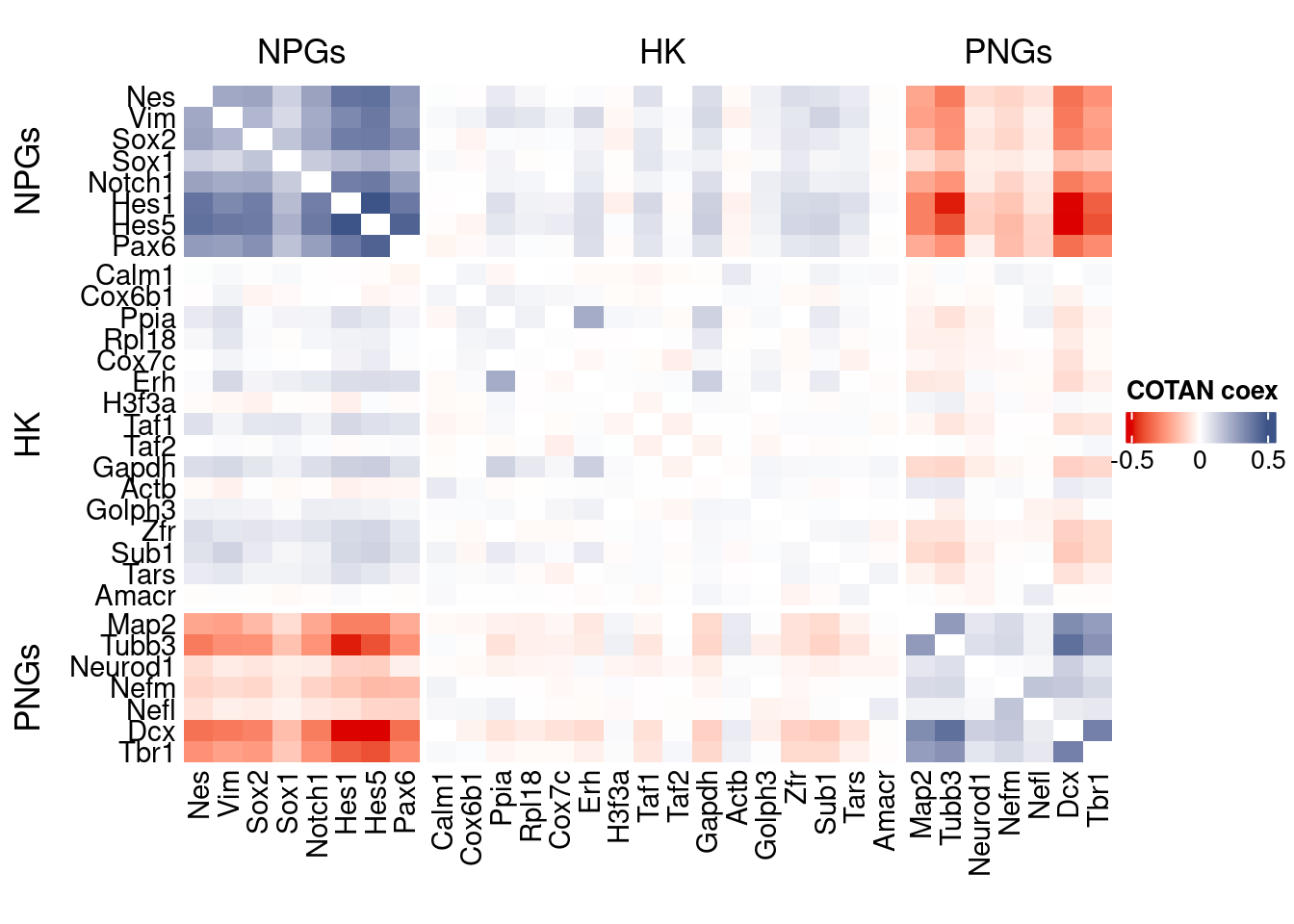
GDI_DF <- calculateGDI(obj)
GDI_DF$geneType <- NA
for (cat in names(genesList)) {
  GDI_DF[rownames(GDI_DF) %in% genesList[[cat]],]$geneType <- cat
}

GDI_DF$GDI_centered <- scale(GDI_DF$GDI,center = T,scale = T)

GDI_DF[genesFromListExpressed,]
sum.raw.norm GDI exp.cells geneType GDI_centered
Nes 7.581052 4.192489 25.4165830 NPGs 3.04415531
Vim 9.971694 3.984104 76.6512748 NPGs 2.75607580
Sox2 7.082317 3.999433 18.5304156 NPGs 2.77726729
Sox1 5.715170 2.983572 5.6615138 NPGs 1.37290505
Notch1 7.227078 3.984877 20.6384260 NPGs 2.75714514
Hes1 8.449033 4.822367 31.8409958 NPGs 3.91492097
Hes5 9.585092 4.784038 42.6018872 NPGs 3.86193346
Pax6 8.481894 4.385577 44.5492873 NPGs 3.31108627
Map2 9.355155 3.931909 70.5681590 PNGs 2.68391910
Tubb3 10.986131 4.374838 76.9524192 PNGs 3.29624084
Neurod1 5.123468 2.046275 2.8508332 PNGs 0.07715236
Nefm 5.862676 3.085697 5.9024292 PNGs 1.51408601
Nefl 4.741106 2.586671 1.8871713 PNGs 0.82421512
Dcx 8.357463 4.539183 39.6707488 PNGs 3.52343659
Tbr1 7.759295 4.237369 26.0991769 PNGs 3.10619909
Calm1 10.447080 1.385779 97.8919896 hk -0.83594052
Cox6b1 9.981533 1.441202 96.6673359 hk -0.75932183
Ppia 10.196964 2.609030 86.8901827 hk 0.85512419
Rpl18 10.790428 1.335148 99.6386268 hk -0.90593539
Cox7c 10.031070 1.518121 97.1893194 hk -0.65298677
Erh 9.280735 2.711007 67.8377836 hk 0.99610081
H3f3a 10.665312 1.380775 99.6587031 hk -0.84285899
Taf1 6.937213 2.168233 17.1049990 hk 0.24575162
Taf2 6.537627 1.310694 12.1863080 hk -0.93974092
Gapdh 9.979987 2.531673 92.7323831 hk 0.74818409
Actb 11.323008 1.382499 99.4980928 hk -0.84047559
Golph3 6.990454 1.648246 19.0724754 hk -0.47309720
Zfr 8.192974 2.212476 47.4001205 hk 0.30691375
Sub1 9.735618 2.343091 92.1903232 hk 0.48748156
Tars 6.946500 1.753805 17.9682795 hk -0.32716939
Amacr 5.143626 1.632567 3.4932744 hk -0.49477252
Reln 7.550123 3.069353 8.3718129 layers 1.49149142
Lhx5 4.850935 2.291750 1.5057217 layers 0.41650600
Cux1 8.229655 3.634065 43.1840996 layers 2.27216946
Satb2 7.683171 3.401215 21.5418591 layers 1.95026951
Tle1 7.461375 2.108275 25.6976511 layers 0.16286267
Mef2c 7.773242 3.876656 19.5543064 layers 2.60753655
Rorb 6.274757 1.635946 7.5486850 layers -0.49010169
Sox5 9.709193 3.707954 64.7460349 layers 2.37431668
Bcl11b 8.848123 4.654283 43.7060831 layers 3.68255551
Fezf2 8.690887 2.925436 54.6878137 layers 1.29253570
Foxp2 7.803267 2.713967 28.2674162 layers 1.00019356
Ntf3 5.006960 2.463725 2.2485445 layers 0.65424957
Cux2 6.681962 2.670967 9.2551696 layers 0.94074878
Slc17a6 7.136129 3.316106 14.1337081 layers 1.83261146
Sema3c 6.576389 2.740901 8.7733387 layers 1.03742781
Thsd7a 4.705115 1.784039 1.3451114 layers -0.28537229
Sulf2 5.293881 2.461288 3.2523590 layers 0.65088105
Kcnk2 7.401683 1.957314 21.6422405 layers -0.04583116
Grik3 5.864890 3.353295 5.0793013 layers 1.88402330
Etv1 5.600431 2.460104 4.1758683 layers 0.64924346
Tle4 6.694944 1.811217 12.5276049 layers -0.24780084
Tmem200a 4.701951 2.381286 1.8068661 layers 0.54028368
Glra2 6.044741 3.654254 5.6414375 layers 2.30007960
Etv1.1 5.600431 2.460104 4.1758683 layers 0.64924346
Sulf1 4.529211 2.076179 0.9235093 layers 0.11849227
Syt6 5.144411 2.559922 2.6902228 layers 0.78723640GDIPlot(obj,GDIIn = GDI_DF, genes = genesList,GDIThreshold = 1.4)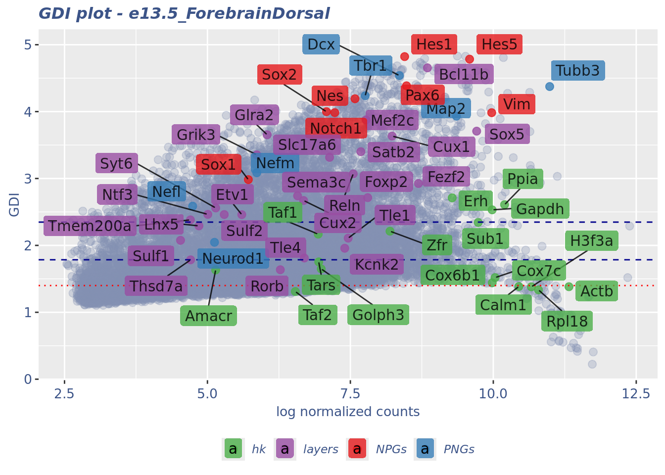
Seurat correlation
srat<- CreateSeuratObject(counts = getRawData(obj),
                          project = project,
                          min.cells = 3,
                          min.features = 200)
srat[["percent.mt"]] <- PercentageFeatureSet(srat, pattern = "^mt-")
srat <- NormalizeData(srat)
srat <- FindVariableFeatures(srat, selection.method = "vst", nfeatures = 2000)

# plot variable features with and without labels
plot1 <- VariableFeaturePlot(srat)

plot1$data$centered_variance <- scale(plot1$data$variance.standardized,
                                      center = T,scale = F)

write.csv(plot1$data,paste0("CoexData/",
                            "Variance_Seurat_genes",
                            getMetadataElement(obj,
                                               datasetTags()[["cond"]]),".csv"))

LabelPoints(plot = plot1, points = c(genesList$NPGs,genesList$PNGs,genesList$layers), repel = TRUE)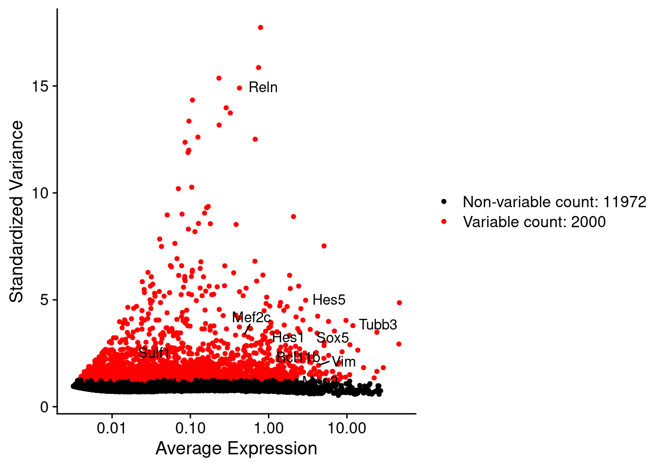
LabelPoints(plot = plot1, points = c(genesList$hk), repel = TRUE)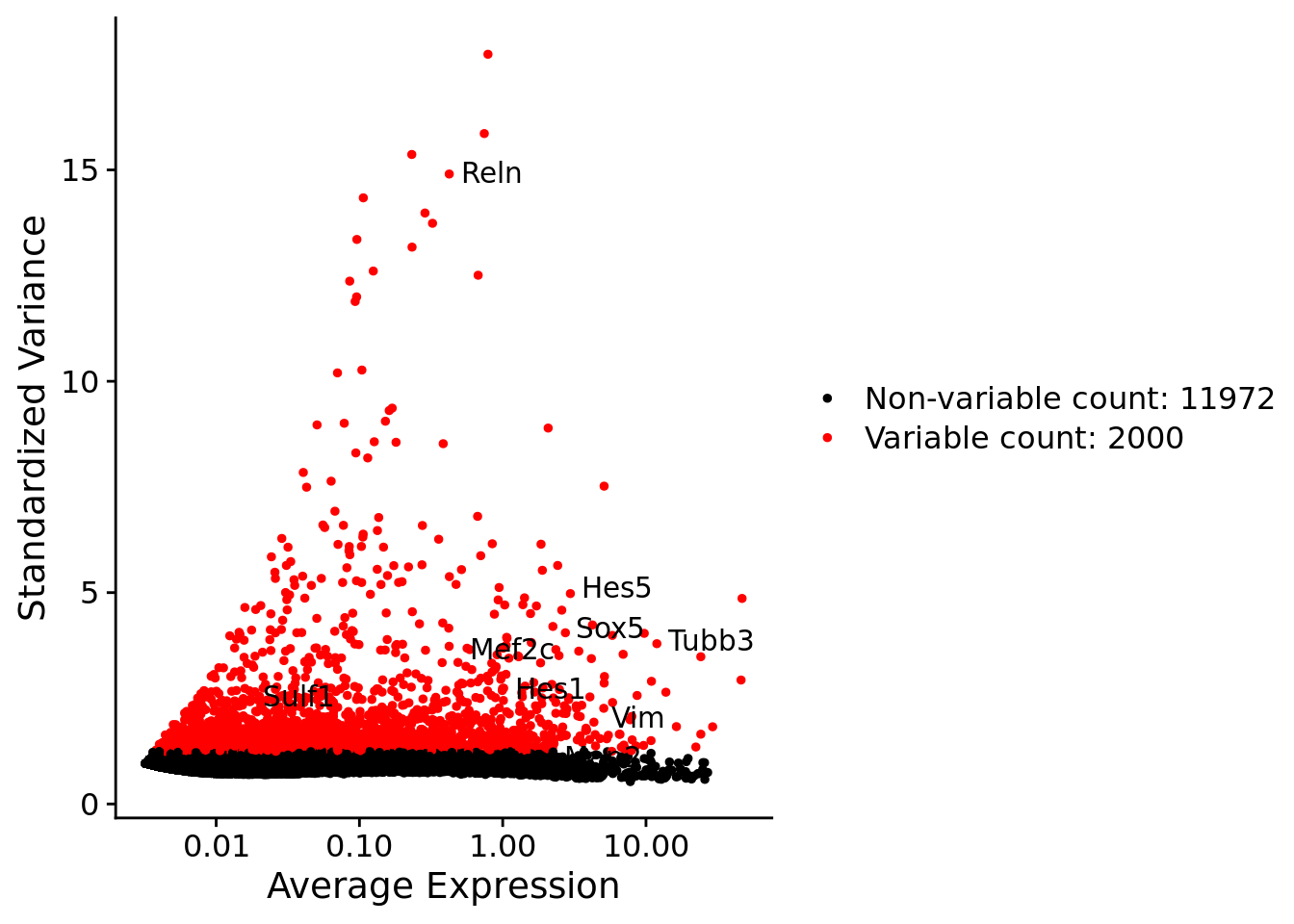
all.genes <- rownames(srat)
srat <- ScaleData(srat, features = all.genes)
seurat.data = GetAssayData(srat[["RNA"]],layer = "data")
corr.pval.list <- correlation_pvalues(data = seurat.data,
genesFromListExpressed,
n.cells = getNumCells(obj))
seurat.data.cor.big <- as.matrix(Matrix::forceSymmetric(corr.pval.list$data.cor, uplo = "U"))
htmp <- correlation_plot(seurat.data.cor.big,
genesList, title="Seurat corr")
p_values.fromSeurat <- corr.pval.list$p_values
seurat.data.cor.big <- corr.pval.list$data.cor
rm(corr.pval.list)
gc() used (Mb) gc trigger (Mb) max used (Mb)
Ncells 10167047 543.0 17751414 948.1 17751414 948.1
Vcells 260464416 1987.2 610438294 4657.3 762094001 5814.4draw(htmp, heatmap_legend_side="right")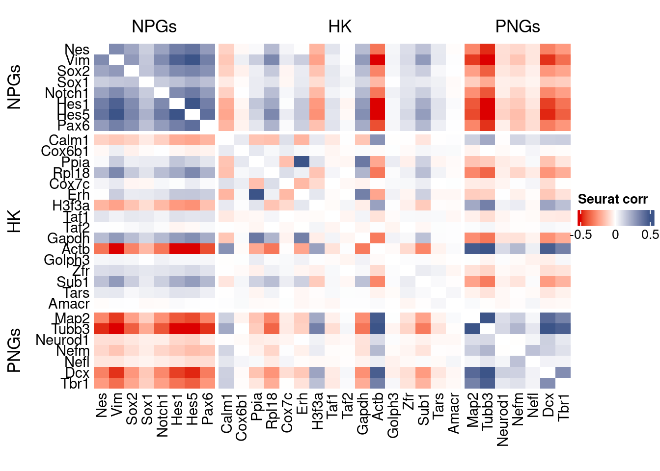
rm(seurat.data.cor.big)
rm(p_values.fromSeurat)
Seurat SC Transform
srat <-  SCTransform(srat,
                     method = "glmGamPoi",
                     vars.to.regress = "percent.mt",
                     verbose = FALSE)

seurat.data <- GetAssayData(srat[["SCT"]],layer = "data")

#Remove genes with all zeros
seurat.data <-seurat.data[rowSums(seurat.data) > 0,]


corr.pval.list <- correlation_pvalues(seurat.data,
                                      genesFromListExpressed,
                                      n.cells = getNumCells(obj))


seurat.data.cor.big <- as.matrix(Matrix::forceSymmetric(corr.pval.list$data.cor, uplo = "U"))

htmp <- correlation_plot(seurat.data.cor.big,
                         genesList, title="Seurat corr SCT")


p_values.fromSeurat <- corr.pval.list$p_values
seurat.data.cor.big <- corr.pval.list$data.cor

rm(corr.pval.list)
gc()
used (Mb) gc trigger (Mb) max used (Mb)
Ncells 10495561 560.6 17751414 948.1 17751414 948.1
Vcells 310497134 2369.0 610438294 4657.3 762094001 5814.4draw(htmp, heatmap_legend_side="right")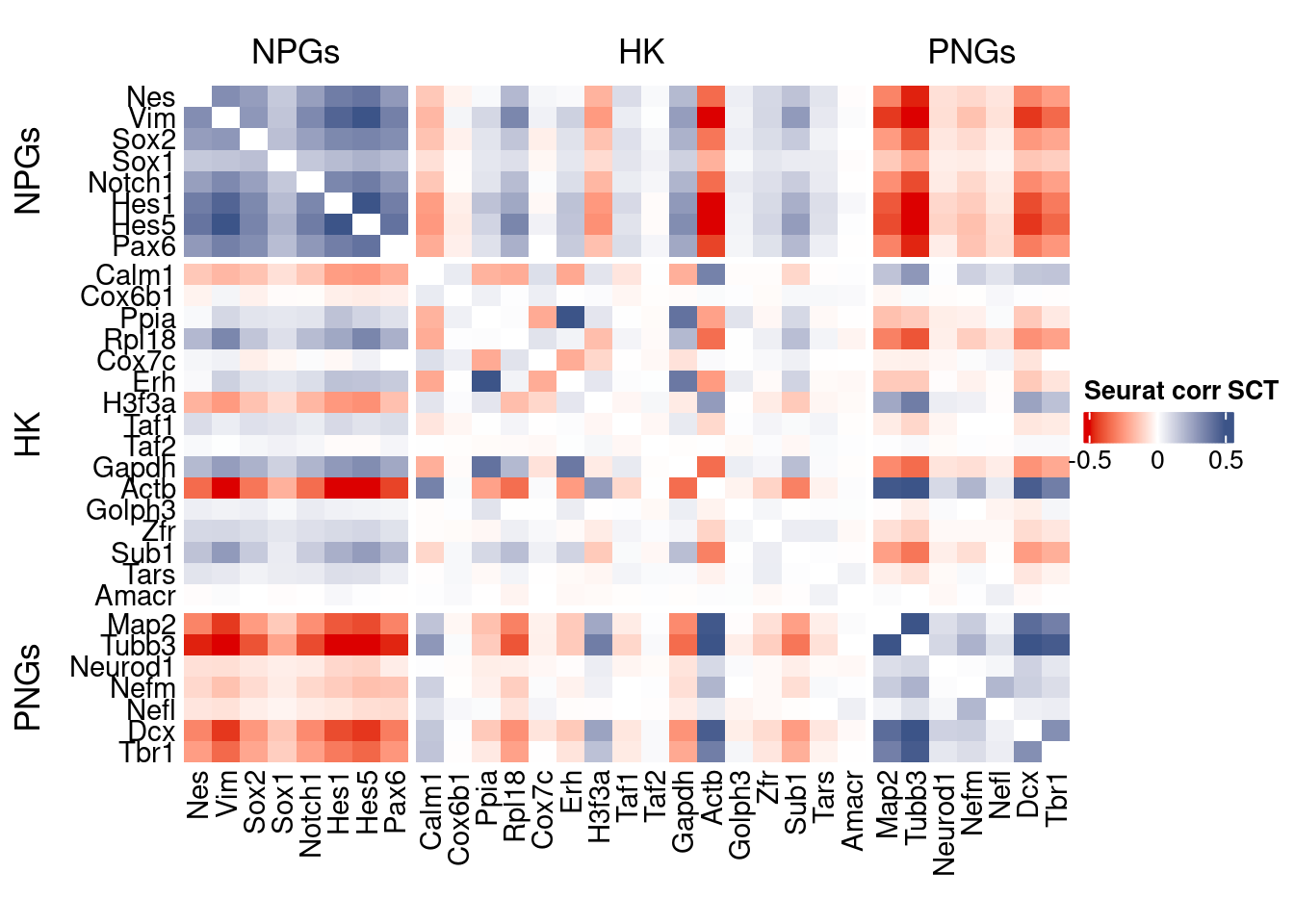
plot1 <- VariableFeaturePlot(srat)

plot1$data$centered_variance <- scale(plot1$data$residual_variance,
center = T,scale = F)write.csv(plot1$data,paste0("CoexData/",
"Variance_SeuratSCT_genes",
getMetadataElement(obj,
datasetTags()[["cond"]]),".csv"))
write_fst(as.data.frame(seurat.data.cor.big),path = paste0("CoexData/SeuratCorrSCT_",file_code,".fst"), compress = 100)
write_fst(as.data.frame(p_values.fromSeurat),path = paste0("CoexData/SeuratPValuesSCT_", file_code,".fst"))
write.csv(as.data.frame(p_values.fromSeurat),paste0("CoexData/SeuratPValuesSCT_", file_code,".csv"))
rm(seurat.data.cor.big)
rm(p_values.fromSeurat)Monocle
library(monocle3)cds <- new_cell_data_set(getRawData(obj),
cell_metadata = getMetadataCells(obj),
gene_metadata = getMetadataGenes(obj)
)
cds <- preprocess_cds(cds, num_dim = 100)
normalized_counts <- normalized_counts(cds)#Remove genes with all zeros
normalized_counts <- normalized_counts[rowSums(normalized_counts) > 0,]
corr.pval.list <- correlation_pvalues(normalized_counts,
genesFromListExpressed,
n.cells = getNumCells(obj))
rm(normalized_counts)
monocle.data.cor.big <- as.matrix(Matrix::forceSymmetric(corr.pval.list$data.cor, uplo = "U"))
htmp <- correlation_plot(data.cor.big = monocle.data.cor.big,
genesList,
title = "Monocle corr")
p_values.from.monocle <- corr.pval.list$p_values
monocle.data.cor.big <- corr.pval.list$data.cor
rm(corr.pval.list)
gc() used (Mb) gc trigger (Mb) max used (Mb)
Ncells 10681826 570.5 17751414 948.1 17751414 948.1
Vcells 312749819 2386.1 610438294 4657.3 762094001 5814.4draw(htmp, heatmap_legend_side="right")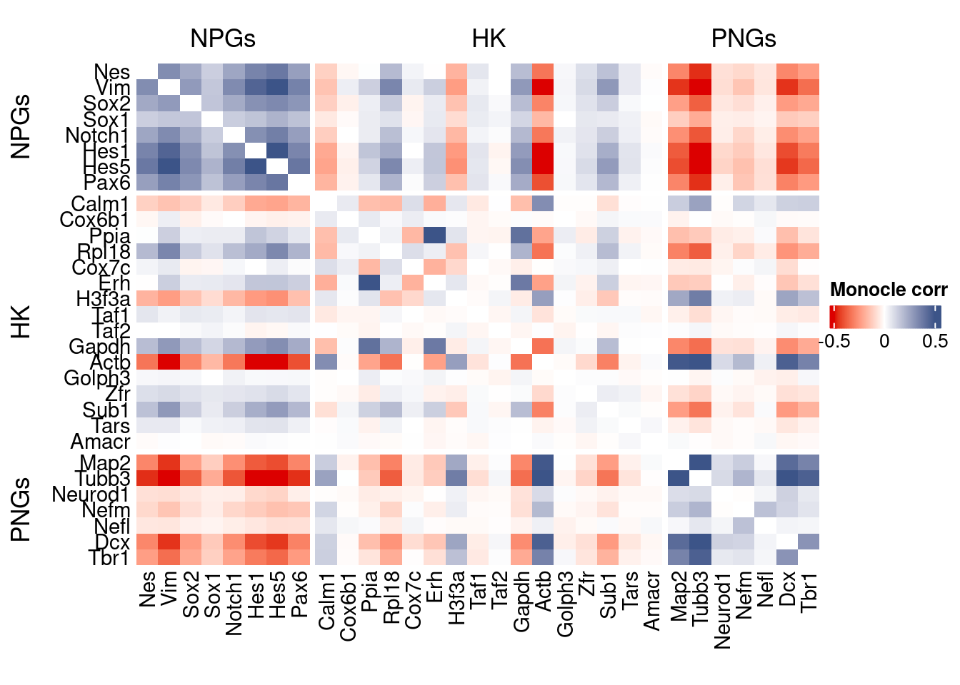
Cs-Core
library(CSCORE)Convert to Seurat obj
sceObj <- convertToSingleCellExperiment(obj)

# Correct: assay=NULL (or omit), data=NULL (since no logcounts)
seuratObj <- as.Seurat(
  x       = sceObj,
  counts  = "counts",
  data    = NULL,
  assay   = NULL,      # IMPORTANT: do NOT set to "RNA" here
  project = "COTAN"
)

# as.Seurat(SCE) creates assay "originalexp" by default; rename it to RNA
seuratObj <- RenameAssays(seuratObj, originalexp = "RNA", verbose = FALSE)
DefaultAssay(seuratObj) <- "RNA"

# Optional: keep COTAN payload
seuratObj@misc$COTAN <- S4Vectors::metadata(sceObj)
Extract CS_CORE corr matrix
#seuratObj@assays$RNA@counts <- ceiling(seuratObj@assays$RNA@counts)
csCoreRes <- CSCORE(seuratObj, genes = genesFromListExpressed)
[INFO] IRLS converged after 2 iterations.
[INFO] Starting WLS for covariance at Wed Jan 21 10:13:59 2026
[INFO] 0.1253% co-expression estimates were greater than 1 and were set to 1.
[INFO] 0.0000% co-expression estimates were smaller than -1 and were set to -1.
[INFO] Finished WLS. Elapsed time: 0.1212 seconds.mat <- as.matrix(csCoreRes$est)
diag(mat) <- 0
split.genes <- base::factor(c(rep("NPGs",sum(genesList[["NPGs"]] %in% genesFromListExpressed)),
rep("HK",sum(genesList[["hk"]] %in% genesFromListExpressed)),
rep("PNGs",sum(genesList[["PNGs"]] %in% genesFromListExpressed))
),
levels = c("NPGs","HK","PNGs"))
f1 = colorRamp2(seq(-0.5,0.5, length = 3), c("#DC0000B2", "white","#3C5488B2" ))
htmp <- Heatmap(as.matrix(mat[c(genesList$NPGs,genesList$hk,genesList$PNGs),c(genesList$NPGs,genesList$hk,genesList$PNGs)]),
#width = ncol(coexMat)*unit(2.5, "mm"),
height = nrow(mat)*unit(3, "mm"),
cluster_rows = FALSE,
cluster_columns = FALSE,
col = f1,
row_names_side = "left",
row_names_gp = gpar(fontsize = 11),
column_names_gp = gpar(fontsize = 11),
column_split = split.genes,
row_split = split.genes,
cluster_row_slices = FALSE,
cluster_column_slices = FALSE,
heatmap_legend_param = list(
title = "CS-CORE", at = c(-0.5, 0, 0.5),
direction = "horizontal",
labels = c("-0.5", "0", "0.5")
)
)
draw(htmp, heatmap_legend_side="right")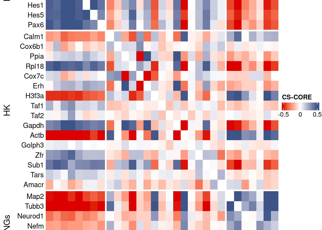
Save CS_CORE matrix
write_fst(as.data.frame(csCoreRes$est), path = paste0("CoexData/CS_CORECorr_", file_code,".fst"),compress = 100)
write_fst(as.data.frame(csCoreRes$p_value), path = paste0("CoexData/CS_COREPValues_", file_code,".fst"),compress = 100)
write.csv(as.data.frame(csCoreRes$p_value), paste0("CoexData/CS_COREPValues_", file_code,".csv"))
Baseline: Spearman on UMI counts
corr.pval.list <- correlation_pvaluesSpearman(data = getRawData(obj),
                                      genesFromListExpressed,
                                      n.cells = getNumCells(obj))

data.cor.big <- as.matrix(Matrix::forceSymmetric(corr.pval.list$data.cor, uplo = "U"))

htmp <- correlation_plot(data.cor.big,
                         genesList, title="UMI baseline S. corr")


p_values.fromSp.C <- corr.pval.list$p_values
data.cor.bigSp.C <- corr.pval.list$data.cor

rm(corr.pval.list)
gc()
used (Mb) gc trigger (Mb) max used (Mb)
Ncells 10690537 571.0 17751414 948.1 17751414 948.1
Vcells 313072530 2388.6 610438294 4657.3 762094001 5814.4draw(htmp, heatmap_legend_side="right")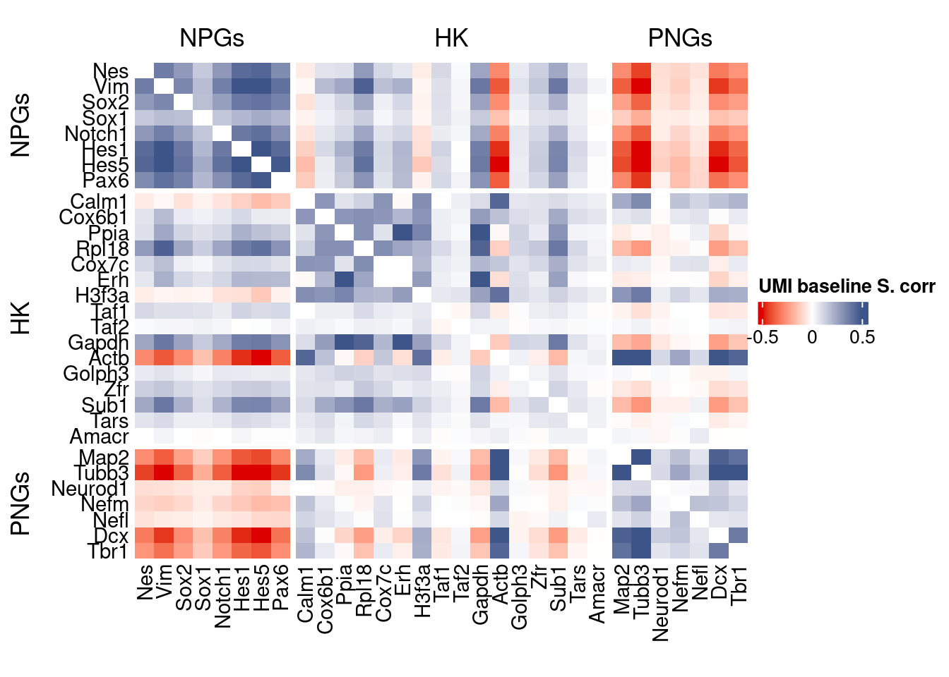
write.csv(as.data.frame(p_values.fromSp.C), paste0("CoexData/BaselineUMISpCorrPValues_", file_code,".csv"))Baseline: Pearson on binarized counts
corr.pval.list <- correlation_pvalues(data = getZeroOneProj(obj),
                                      genesFromListExpressed,
                                      n.cells = getNumCells(obj))

data.cor.big <- as.matrix(Matrix::forceSymmetric(corr.pval.list$data.cor, uplo = "U"))

htmp <- correlation_plot(data.cor.big,
                         genesList, title="Zero-one P. corr")


p_values.fromSp.C <- corr.pval.list$p_values
data.cor.bigSp.C <- corr.pval.list$data.cor

rm(corr.pval.list)
gc()
used (Mb) gc trigger (Mb) max used (Mb)
Ncells 10690664 571.0 17751414 948.1 17751414 948.1
Vcells 313072787 2388.6 610438294 4657.3 762094001 5814.4draw(htmp, heatmap_legend_side="right")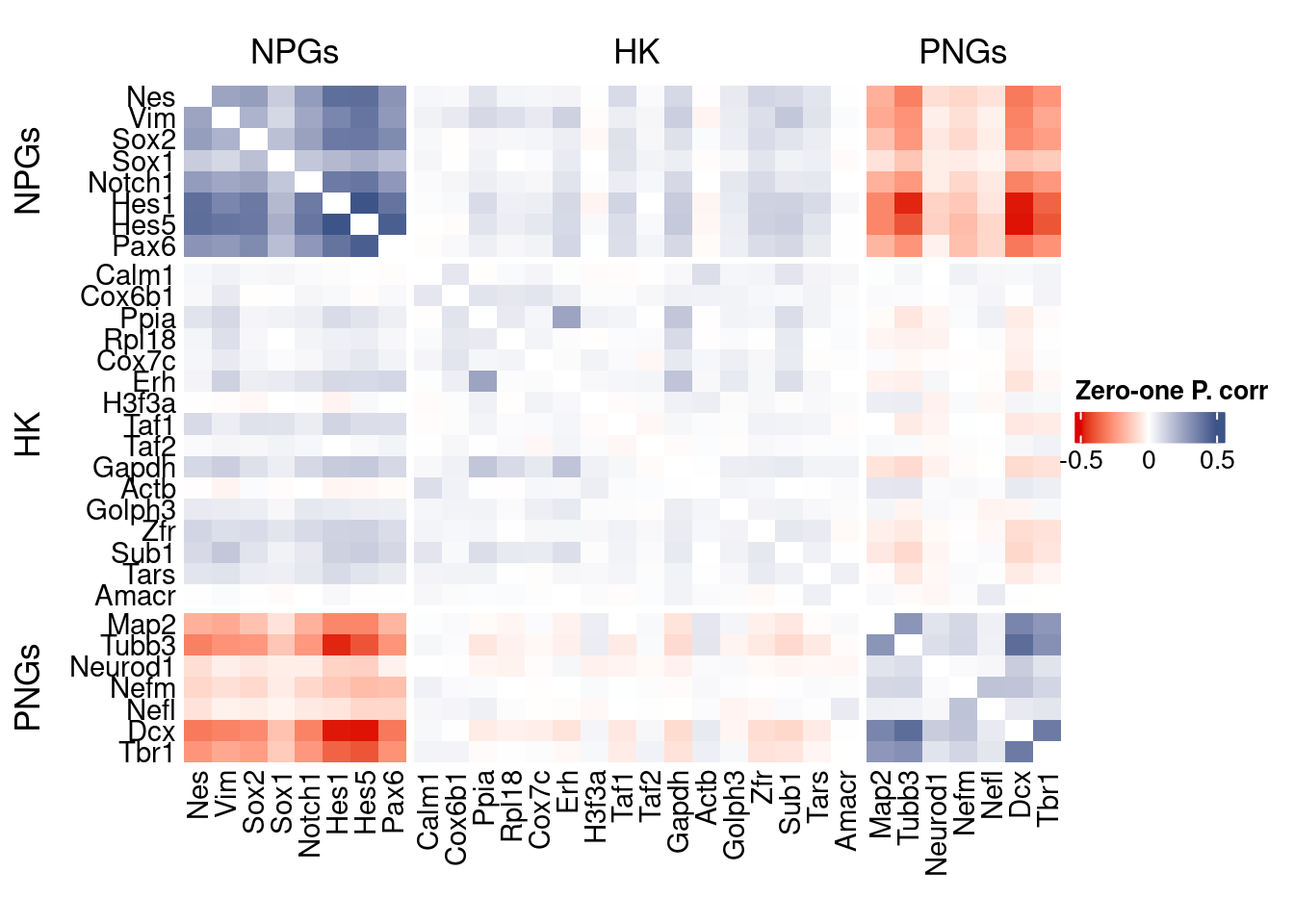
write.csv(as.data.frame(p_values.fromSp.C), paste0("CoexData/ZeroOnePCorrPValues_", file_code,".csv"))Sys.time()[1] "2026-01-21 10:14:05 CET"sessionInfo()R version 4.5.2 (2025-10-31)
Platform: x86_64-pc-linux-gnu
Running under: Ubuntu 22.04.5 LTS
Matrix products: default
BLAS: /usr/lib/x86_64-linux-gnu/blas/libblas.so.3.10.0
LAPACK: /usr/lib/x86_64-linux-gnu/lapack/liblapack.so.3.10.0 LAPACK version 3.10.0
locale:
[1] LC_CTYPE=C.UTF-8 LC_NUMERIC=C LC_TIME=C.UTF-8
[4] LC_COLLATE=C.UTF-8 LC_MONETARY=C.UTF-8 LC_MESSAGES=C.UTF-8
[7] LC_PAPER=C.UTF-8 LC_NAME=C LC_ADDRESS=C
[10] LC_TELEPHONE=C LC_MEASUREMENT=C.UTF-8 LC_IDENTIFICATION=C
time zone: Europe/Rome
tzcode source: system (glibc)
attached base packages:
[1] stats4 parallel grid stats graphics grDevices utils
[8] datasets methods base
other attached packages:
[1] CSCORE_1.0.2 monocle3_1.3.7
[3] SingleCellExperiment_1.32.0 SummarizedExperiment_1.38.1
[5] GenomicRanges_1.62.1 Seqinfo_1.0.0
[7] IRanges_2.44.0 S4Vectors_0.48.0
[9] MatrixGenerics_1.22.0 matrixStats_1.5.0
[11] Biobase_2.70.0 BiocGenerics_0.56.0
[13] generics_0.1.3 fstcore_0.10.0
[15] fst_0.9.8 stringr_1.6.0
[17] HiClimR_2.2.1 doParallel_1.0.17
[19] iterators_1.0.14 foreach_1.5.2
[21] Rfast_2.1.5.1 RcppParallel_5.1.10
[23] zigg_0.0.2 Rcpp_1.1.0
[25] patchwork_1.3.2 Seurat_5.4.0
[27] SeuratObject_5.3.0 sp_2.2-0
[29] Hmisc_5.2-3 dplyr_1.1.4
[31] circlize_0.4.16 ComplexHeatmap_2.26.0
[33] COTAN_2.11.1
loaded via a namespace (and not attached):
[1] RcppAnnoy_0.0.22 splines_4.5.2
[3] later_1.4.2 tibble_3.3.0
[5] polyclip_1.10-7 rpart_4.1.24
[7] fastDummies_1.7.5 lifecycle_1.0.4
[9] Rdpack_2.6.4 globals_0.18.0
[11] lattice_0.22-7 MASS_7.3-65
[13] backports_1.5.0 ggdist_3.3.3
[15] dendextend_1.19.0 magrittr_2.0.4
[17] plotly_4.11.0 rmarkdown_2.29
[19] yaml_2.3.10 httpuv_1.6.16
[21] otel_0.2.0 glmGamPoi_1.20.0
[23] sctransform_0.4.2 spam_2.11-1
[25] spatstat.sparse_3.1-0 reticulate_1.44.1
[27] minqa_1.2.8 cowplot_1.2.0
[29] pbapply_1.7-2 RColorBrewer_1.1-3
[31] abind_1.4-8 Rtsne_0.17
[33] purrr_1.2.0 nnet_7.3-20
[35] GenomeInfoDbData_1.2.14 ggrepel_0.9.6
[37] irlba_2.3.5.1 listenv_0.10.0
[39] spatstat.utils_3.2-1 goftest_1.2-3
[41] RSpectra_0.16-2 spatstat.random_3.4-3
[43] fitdistrplus_1.2-2 parallelly_1.46.0
[45] DelayedMatrixStats_1.30.0 ncdf4_1.24
[47] codetools_0.2-20 DelayedArray_0.36.0
[49] tidyselect_1.2.1 shape_1.4.6.1
[51] UCSC.utils_1.4.0 farver_2.1.2
[53] lme4_1.1-37 ScaledMatrix_1.16.0
[55] viridis_0.6.5 base64enc_0.1-3
[57] spatstat.explore_3.6-0 jsonlite_2.0.0
[59] GetoptLong_1.1.0 Formula_1.2-5
[61] progressr_0.18.0 ggridges_0.5.6
[63] survival_3.8-3 tools_4.5.2
[65] ica_1.0-3 glue_1.8.0
[67] gridExtra_2.3 SparseArray_1.10.8
[69] xfun_0.52 distributional_0.6.0
[71] ggthemes_5.2.0 GenomeInfoDb_1.44.0
[73] withr_3.0.2 fastmap_1.2.0
[75] boot_1.3-32 digest_0.6.37
[77] rsvd_1.0.5 parallelDist_0.2.6
[79] R6_2.6.1 mime_0.13
[81] colorspace_2.1-1 Cairo_1.7-0
[83] scattermore_1.2 tensor_1.5
[85] spatstat.data_3.1-9 tidyr_1.3.1
[87] data.table_1.18.0 httr_1.4.7
[89] htmlwidgets_1.6.4 S4Arrays_1.10.1
[91] uwot_0.2.3 pkgconfig_2.0.3
[93] gtable_0.3.6 lmtest_0.9-40
[95] S7_0.2.1 XVector_0.50.0
[97] htmltools_0.5.8.1 dotCall64_1.2
[99] clue_0.3-66 scales_1.4.0
[101] png_0.1-8 reformulas_0.4.1
[103] spatstat.univar_3.1-6 rstudioapi_0.18.0
[105] knitr_1.50 reshape2_1.4.4
[107] rjson_0.2.23 nloptr_2.2.1
[109] checkmate_2.3.2 nlme_3.1-168
[111] proxy_0.4-29 zoo_1.8-14
[113] GlobalOptions_0.1.2 KernSmooth_2.23-26
[115] miniUI_0.1.2 foreign_0.8-90
[117] pillar_1.11.1 vctrs_0.7.0
[119] RANN_2.6.2 promises_1.5.0
[121] BiocSingular_1.26.1 beachmat_2.26.0
[123] xtable_1.8-4 cluster_2.1.8.1
[125] htmlTable_2.4.3 evaluate_1.0.5
[127] magick_2.9.0 zeallot_0.2.0
[129] cli_3.6.5 compiler_4.5.2
[131] rlang_1.1.7 crayon_1.5.3
[133] future.apply_1.20.0 labeling_0.4.3
[135] plyr_1.8.9 stringi_1.8.7
[137] viridisLite_0.4.2 deldir_2.0-4
[139] BiocParallel_1.44.0 assertthat_0.2.1
[141] lazyeval_0.2.2 spatstat.geom_3.6-1
[143] Matrix_1.7-4 RcppHNSW_0.6.0
[145] sparseMatrixStats_1.20.0 future_1.69.0
[147] ggplot2_4.0.1 shiny_1.12.1
[149] rbibutils_2.3 ROCR_1.0-11
[151] igraph_2.2.1