library(assertthat)
library(rlang)
library(scales)
library(ggplot2)
library(zeallot)
library(data.table)
library(parallelDist)
library(tidyr)
library(tidyverse)
library(ggh4x)
library(gridExtra)

#options(parallelly.fork.enable = TRUE)

inDir <- file.path("Results")

#setLoggingLevel(2)
#setLoggingFile(file.path(inDir, "MixingClustersGDI_ForebrainDorsal.log"))

outDir <- file.path(inDir, "GDI_Sensitivity")
if (!file.exists(outDir)) {
  dir.create(outDir)
}GDI Increment From Mixing
Preamble
Re-Load calculated data for analysis
Define all mixing fractions
allMixingFractions <- c(0.05, 0.10, 0.20, 0.40, 0.80)
names(allMixingFractions) <-
  str_pad(scales::label_percent()(allMixingFractions), 3, pad = "0")
Actually load the data
allResList <-
  lapply(
    names(allMixingFractions),
    function(mixStr) {
      readRDS(file.path(outDir, paste0("GDI_with_", mixStr, "_Mixing.RDS")))
    })
names(allResList) <- names(allMixingFractions)

assert_that(unique(sapply(allResList, ncol)) == 5L)
[1] TRUEAdd baseline (“00%” mixing)
baseline <- allResList[[1L]]

baseline[["MixingFraction"]] <- 0.0
baseline[["GDI"]] <- baseline[["GDI"]] - baseline[["GDIIncrement"]]
baseline[["GDIIncrement"]] <- 0.0

allResListWithBase <- append(list("00%" = baseline), allResList)

rm(baseline)
Merge all results and calculate the fitting regression for each cluster pair
allRes <-
  cbind(allResList[[1L]][, 1:2],
        lapply(allResList, function(df) { df[, 3:5] }))

colnames(allRes) <-
  c(colnames(allResList[[1L]])[1:2],
    paste0(
      rep(colnames(allResList[[1L]])[3:5], 5),
      "_",
      rep(names(allMixingFractions), each = 3)
    )
  )

allResWithBase <-
  cbind(allResListWithBase[[1L]][, 1:2],
        lapply(allResListWithBase, function(df) { df[, 3:5] }))

colnames(allResWithBase) <-
  c(colnames(allResListWithBase[[1L]])[1:2],
    paste0(
      rep(colnames(allResListWithBase[[1L]])[3:5], 5),
      "_",
      rep(c("00%", names(allMixingFractions)), each = 3)
    )
  )

assert_that(
  identical(
    allRes, allResWithBase[, str_detect(colnames(allResWithBase),
                                        "00%", negate = TRUE)]
  )
)
[1] TRUERecall cluster distance and add it to the results
zeroOneAvg <- readRDS(file.path(outDir,  "allZeroOne.RDS"))
# zeroOneAvg <- readRDS(file.path(outDir, "distanceZeroOne.RDS"))

distZeroOne <-
  as.matrix(parDist(t(zeroOneAvg), method = "hellinger",
                    diag = TRUE, upper = TRUE))^2

distZeroOneLong <-
  rownames_to_column(as.data.frame(distZeroOne), var = "MainCluster")
distZeroOneLong <-
  pivot_longer(distZeroOneLong,
               cols = !MainCluster,
               names_to = "OtherCluster",
               values_to = "Distance")

distZeroOneLong <-
  as.data.frame(distZeroOneLong[distZeroOneLong[["Distance"]] != 0.0, ])

assert_that(identical(distZeroOneLong[, 1:2], allRes[, 1:2]))
[1] TRUEperm <- order(distZeroOneLong[["Distance"]])Scatter plot of ΔGDI vs Distance
distDF <- cbind(distZeroOneLong[, "Distance", drop = FALSE],
                sqrt(distZeroOneLong[, "Distance", drop = FALSE]))
colnames(distDF) <- c("Distance", "DistanceSqrt")

D2IPlot <- ggplot(cbind(allResList[["20%"]], distDF),
                  aes(x = Distance, y = GDIIncrement)) +
             geom_point() +
             geom_smooth(method = lm, formula = y ~ x)
           # +  xlim(0, 1.5) + ylim(0, 1.5) + coord_fixed()

plot(D2IPlot)
Recall cluster distance and add it to the results
zeroOneAvg <- readRDS(file.path(outDir,  "allZeroOne.RDS"))
# zeroOneAvg <- readRDS(file.path(outDir, "distanceZeroOne.RDS"))

distZeroOne <-
  as.matrix(parDist(t(zeroOneAvg), method = "hellinger",
                    diag = TRUE, upper = TRUE))^2

distZeroOneLong <-
  rownames_to_column(as.data.frame(distZeroOne), var = "MainCluster")
distZeroOneLong <-
  pivot_longer(distZeroOneLong,
               cols = !MainCluster,
               names_to = "OtherCluster",
               values_to = "Distance")

distZeroOneLong <-
  as.data.frame(distZeroOneLong[distZeroOneLong[["Distance"]] != 0.0, ])

assert_that(identical(distZeroOneLong[, 1:2], allRes[, 1:2]))
[1] TRUEperm <- order(distZeroOneLong[["Distance"]])Scatter plot of ΔGDI vs Distance
distDF <- cbind(distZeroOneLong[, "Distance", drop = FALSE],
                sqrt(distZeroOneLong[, "Distance", drop = FALSE]))
colnames(distDF) <- c("Distance", "DistanceSqrt")

D2IPlot <- ggplot(cbind(allResList[["20%"]], distDF),
                  aes(x = Distance, y = GDIIncrement)) +
             geom_point() +
             geom_smooth(method = lm, formula = y ~ x)
           # +  xlim(0, 1.5) + ylim(0, 1.5) + coord_fixed()

plot(D2IPlot)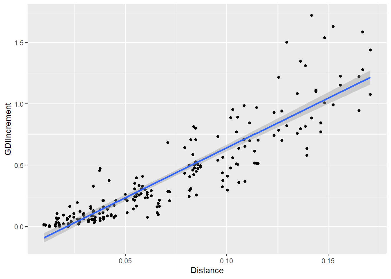
Merge all data and plot it using a-priory (squared) distance as discriminant
allResPerm <-
  do.call(rbind, lapply(allResList, function(df) df[perm, ]))

allResPerm <-
  cbind(allResPerm,
        "ClusterPair" = rep.int(seq_along(perm),
                                length(allResList)),
        "Distance"    = rep(distZeroOneLong[["Distance"]][perm],
                            length(allResList)))
rownames(allResPerm) <- NULL

dim(allResPerm)
[1] 1050 7allResWithBasePerm <-
do.call(rbind,lapply(allResListWithBase, function(df) df[perm, ]))
allResWithBasePerm <-
cbind(allResWithBasePerm,
"ClusterPair" = rep.int(seq_along(perm),
length(allResListWithBase)),
"Distance" = rep(distZeroOneLong[["Distance"]][perm],
length(allResListWithBase)))
rownames(allResWithBasePerm) <- NULL
dim(allResWithBasePerm)[1] 1260 7assert_that(
all.equal(
allResPerm,
allResWithBasePerm[(length(perm) + 1):nrow(allResWithBasePerm), ],
check.attributes = FALSE
),
msg = "Trouble with meshing all res permutated data"
)[1] TRUEPlot all data using the mixing fraction as abscissas and the distance as color
IScPlot <-
  ggplot(allResPerm,
         aes(x = MixingFraction, y = GDIIncrement, color = Distance)
  ) +
  geom_point() +
  scale_color_continuous(type = "viridis") +
  scale_x_log10() +
  labs(
    x = "Ratio between sizes of second and first cluster",
    y = "Top 1% GDI score increment of genes"
  )

plot(IScPlot)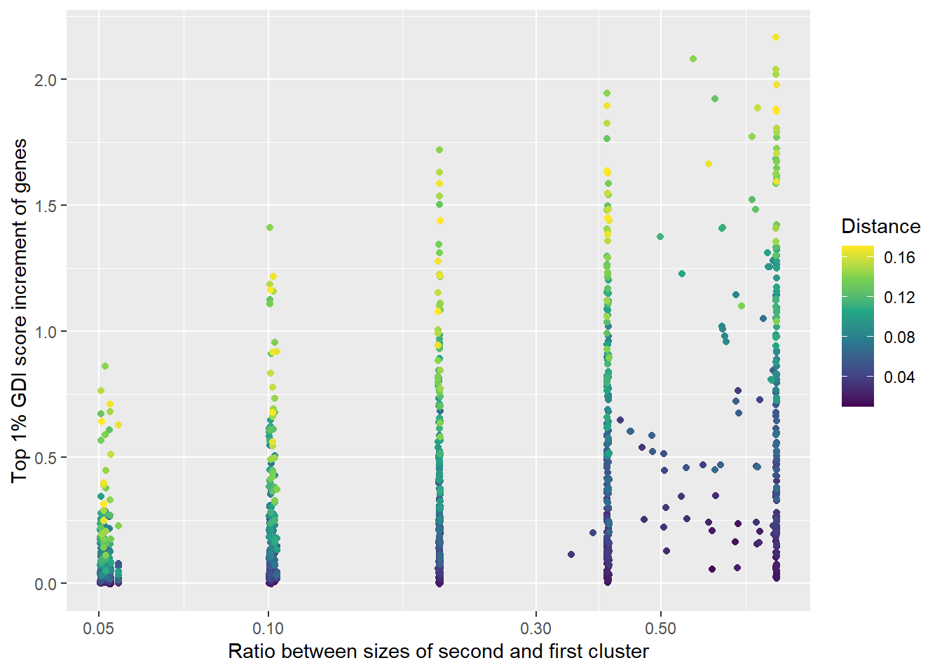
GScPlot <-
  ggplot(allResWithBasePerm,
         aes(x = MixingFraction, y = GDI, color = Distance)
  ) +
  geom_point() +
  scale_color_continuous(type = "viridis") +
  labs(
    x = "Ratio between sizes of second and first cluster",
    y = "Top 1% GDI score of genes"
  )

plot(GScPlot)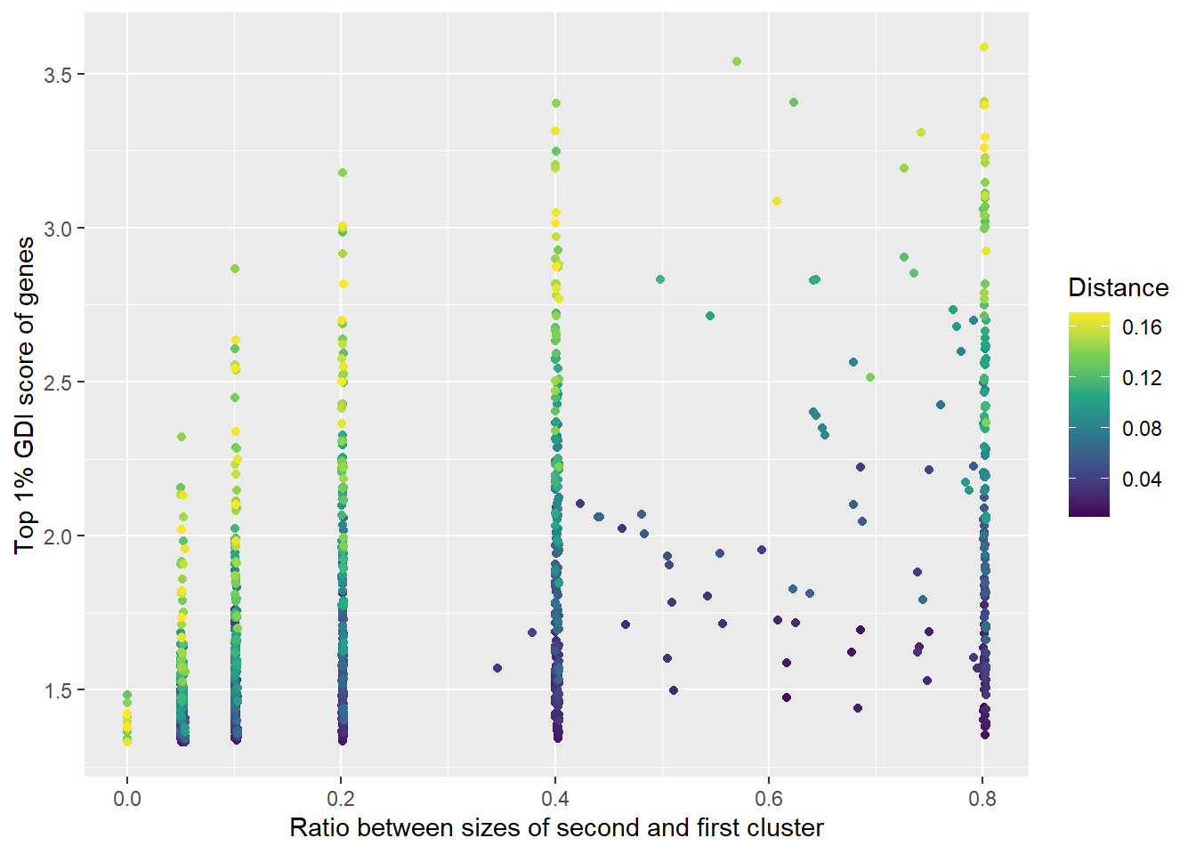
Reorder by cluster pair
reOrder <- function(df, numBlocks) {
  blockLength <- nrow(df) / numBlocks
  permut <- rep(1:blockLength, each = numBlocks) +
              rep(seq(0, nrow(df) - 1, by = blockLength), times = numBlocks)
  return(df[permut, ])
}

allResPerm2 <- reOrder(allResPerm, 5)
allResWithBasePerm2 <- reOrder(allResWithBasePerm, 6)

head(allResPerm[["ClusterPair"]], 20)
[1] 1 2 3 4 5 6 7 8 9 10 11 12 13 14 15 16 17 18 19 20head(allResPerm2[["ClusterPair"]], 20) [1] 1 1 1 1 1 2 2 2 2 2 3 3 3 3 3 4 4 4 4 4Plot by lines
numBuckets <- 6L
bucketLength <- length(perm) %/% numBuckets

ILinesPLot <-
  ggplot(
    allResPerm2,
    aes(x = MixingFraction, y = GDIIncrement,
        color = (ClusterPair - 1) %/% bucketLength + 0.5)
  ) +
  geom_path(aes(group = ClusterPair)) +
  theme(legend.position = "none") +
  scale_colour_stepsn(
    colours = rev(hcl.colors(numBuckets, palette = "Dark 2"))
  ) +
  labs(
    x = "Ratio between sizes of second and first cluster",
    y = "Top 1% GDI score increment of genes"
  )

plot(ILinesPLot)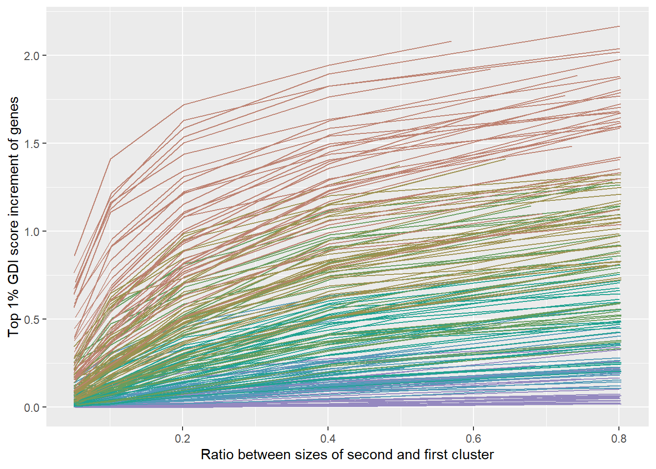
GLinesPLot <-
  ggplot(
    allResWithBasePerm2,
    aes(x = MixingFraction, y = GDI,
        color = (ClusterPair - 1) %/% bucketLength + 0.5)
  ) +
  geom_path(aes(group = ClusterPair)) +
  theme(legend.position = "none") +
  scale_colour_stepsn(
    colours = rev(hcl.colors(numBuckets, palette = "Dark 2"))
  ) +
  labs(
    x = "Ratio between sizes of second and first cluster",
    y = "Top 1% GDI score of genes"
  )

plot(GLinesPLot)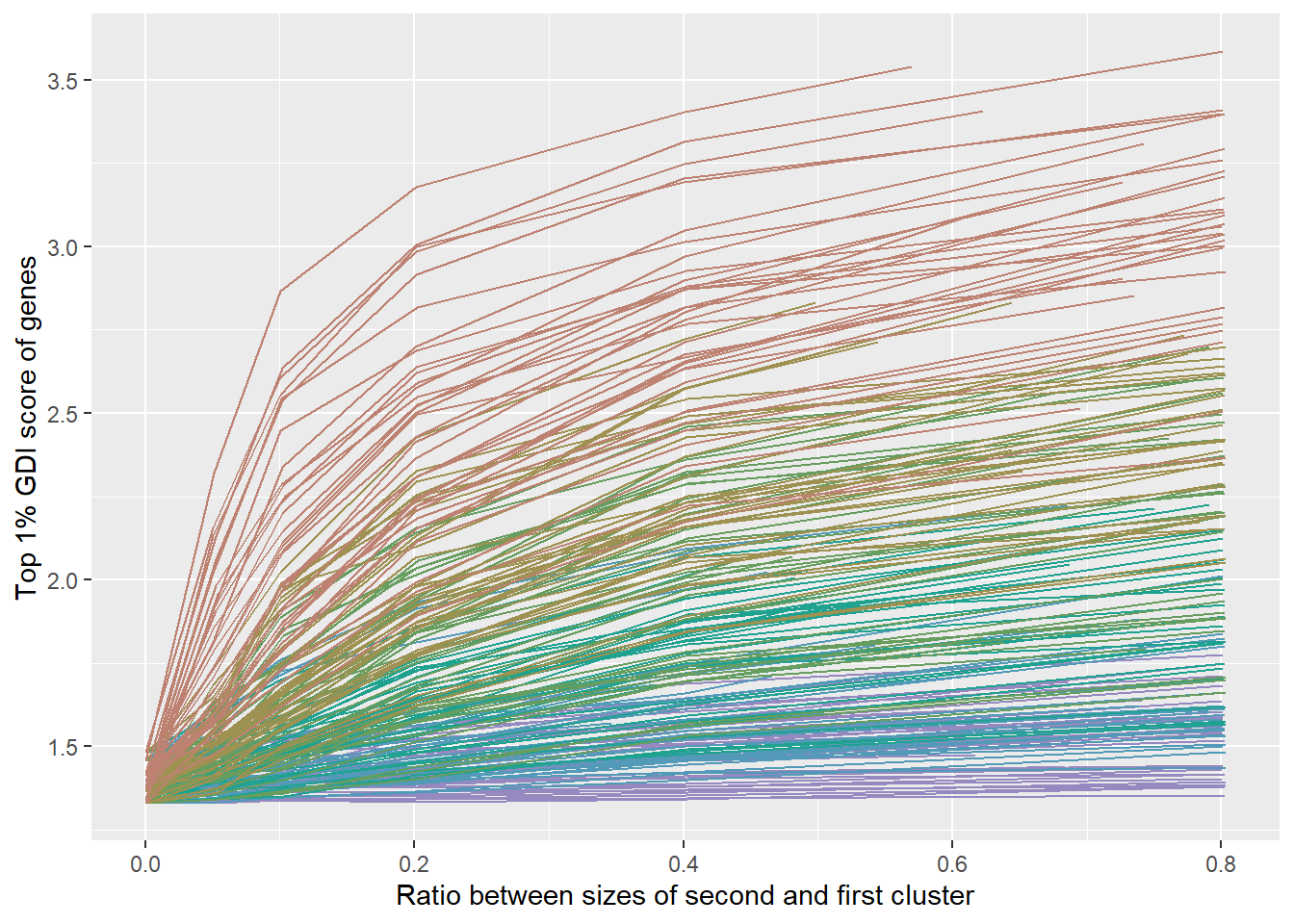
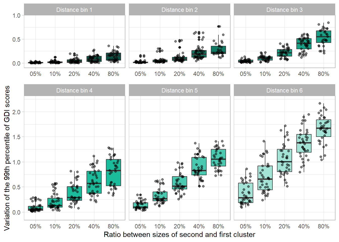
ΔGDI main plot
numBuckets <- 6L
bucketLength <- length(perm) %/% numBuckets

mg <- function(mixings) {
  res <- mixings
  actOn <- res != 0.0
  res[actOn] <- round(log2(res[actOn] * 40))
  return(res)
}

group <- factor((allResPerm[["ClusterPair"]] - 1) %/% bucketLength + 1)
levels(group) <- paste0("Distance bin ", 1:numBuckets)

discreteMixing <- factor(mg(allResPerm[["MixingFraction"]]))
levels(discreteMixing) <- names(allMixingFractions)

allResPermBuck <-
  cbind(allResPerm, "Group" = group, "DiscreteMixing" = discreteMixing)

first.part  <- c("Distance bin 1", "Distance bin 2", "Distance bin 3")
second.part <- c("Distance bin 4", "Distance bin 5", "Distance bin 6")

IBoxPlotA <-
  ggplot(
    allResPermBuck[allResPermBuck[["Group"]] %in% first.part,],
    aes(x = DiscreteMixing, y = GDIIncrement,
        fill = Group, group = DiscreteMixing)
  ) +
  geom_boxplot() +
  geom_jitter(width = 0.25, alpha = 0.5) +
  scale_fill_manual(values = c("#0B5345", "#117A65", "#16A085")) +
  facet_grid2(cols = vars(Group)) +
  scale_y_continuous(
    limits = c(-0.05, 0.95),
    breaks = scales::breaks_width(0.5)
  ) +
  theme_light() +
  theme(legend.position = "none", axis.title.x = element_blank()) +
  labs(
    y = ""
  )

IBoxPlotB <-
  ggplot(
    allResPermBuck[allResPermBuck[["Group"]] %in% second.part, ],
    aes(x = DiscreteMixing, y = GDIIncrement,
        fill = Group, group = DiscreteMixing)
  ) +
  geom_boxplot() +
  geom_jitter(width = 0.25, alpha = 0.5) +
  scale_fill_manual(values = c("#1ABC9C", "#48C9B0", "#A3E4D7")) +
  facet_grid2(cols = vars(Group)) +
  scale_y_continuous(
    limits = c(-0.05, 2.2),
    breaks = scales::breaks_width(0.5)
  ) +
  theme_light() +
  theme(legend.position = "none") +
  labs(
    x = "Ratio between sizes of second and first cluster",
    y = "Variation of the 99th percentile of GDI scores"
  )

finalIPlot <-
  gridExtra::grid.arrange(
    IBoxPlotA, IBoxPlotB, nrow = 3, ncol = 1,
    layout_matrix = cbind(c(1, rep(2, 2)))
  )
grDevices::pdf(file.path(outDir, "GDI-Increment_LaManno_ForebrainDorsal.pdf"),
               width = 7, height = 7)
grid::grid.newpage()
grid::grid.draw(finalIPlot)
grDevices::dev.off()
png
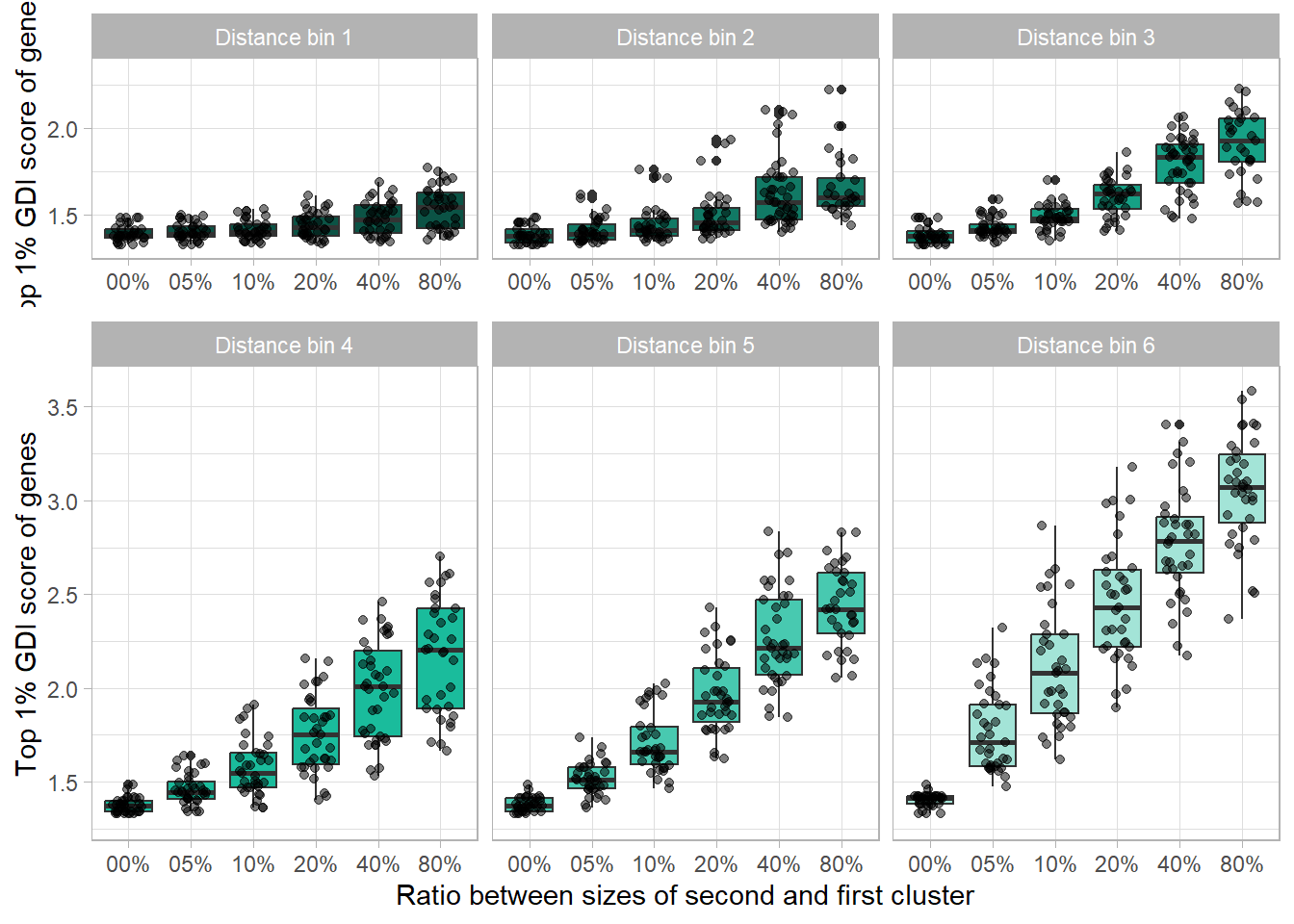
2 GDI main plot
numBuckets <- 6L
bucketLength <- length(perm) %/% numBuckets

mg <- function(mixings) {
  res <- mixings
  actOn <- res != 0.0
  res[actOn] <- round(log2(res[actOn] * 40))
  return(res)
}

group <- factor((allResWithBasePerm[["ClusterPair"]] - 1) %/% bucketLength + 1)
levels(group) <- paste0("Distance bin ", 1:numBuckets)

discreteMixing <- factor(mg(allResWithBasePerm[["MixingFraction"]]))
levels(discreteMixing) <- c("00%", names(allMixingFractions))

allResWithBasePermBuck <-
  cbind(allResWithBasePerm, "Group" = group, "DiscreteMixing" = discreteMixing)

first.part  <- c("Distance bin 1", "Distance bin 2", "Distance bin 3")
second.part <- c("Distance bin 4", "Distance bin 5", "Distance bin 6")


GBoxPlotA <-
  ggplot(
    allResWithBasePermBuck[allResWithBasePermBuck[["Group"]] %in% first.part,],
    aes(x = DiscreteMixing, y = GDI,
        fill = Group, group = DiscreteMixing)
  ) +
  geom_boxplot() +
  geom_jitter(width = 0.25, alpha = 0.5) +
  scale_fill_manual(values = c("#0B5345", "#117A65", "#16A085")) +
  facet_grid2(cols = vars(Group)) +
  scale_y_continuous(
    limits = c(1.30, 2.35),
    breaks = scales::breaks_width(0.5)
  ) +
  theme_light() +
  theme(legend.position = "none", axis.title.x = element_blank()) +
  labs(
    y = "Top 1% GDI score of genes"
  )

GBoxPlotB <-
  ggplot(
    allResWithBasePermBuck[allResWithBasePermBuck[["Group"]] %in% second.part,],
    aes(x = DiscreteMixing, y = GDI,
        fill = Group, group = DiscreteMixing)
  ) +
  geom_boxplot() +
  geom_jitter(width = 0.25, alpha = 0.5) +
  scale_fill_manual(values = c("#1ABC9C", "#48C9B0", "#A3E4D7")) +
  facet_grid2(cols = vars(Group)) +
  scale_y_continuous(
    limits = c(1.30, 3.60),
    breaks = scales::breaks_width(0.5)
  ) +
  theme_light() +
  theme(legend.position = "none") +
  labs(
    x = "Ratio between sizes of second and first cluster",
    y = "Top 1% GDI score of genes"
  )

finalGPlot <-
  gridExtra::grid.arrange(
    GBoxPlotA, GBoxPlotB, nrow = 3, ncol = 1,
    layout_matrix = cbind(c(1, rep(2, 2)))
  )
grDevices::pdf(file.path(outDir, "GDI_LaManno_ForebrainDorsal.pdf"),
               width = 7, height = 7)
grid::grid.newpage()
grid::grid.draw(finalGPlot)
grDevices::dev.off()
png
2 Load calculated data about multi clusters cases for analysis
Compare estimated vs real GDI increment
# Scatter plot of the effective increment [Y] against estimated increment [X]
pg <- ggplot(resMix20_2, aes(x = PredictedGDIIncrement, y = GDIIncrement)) +
  geom_point() +
  geom_smooth(method=lm, formula = y ~ x + 0) +
  coord_fixed() +
  xlim(0, 1.5) + ylim(0, 1.5) +
  labs(
    x = "Predicted - variation of the 99th percentile of GDI scores",
    y = "Observed - variation of the 99th percentile of GDI scores"
  )

plot(pg)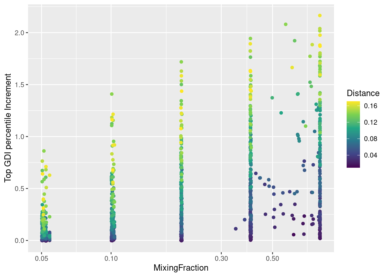
pdf(file.path(outDir, "Estimated-vs-Real_GDI-Increment.pdf"),
               width = 7, height = 7)
plot(pg)
dev.off()
png
2 The plot shows that having the 20% extraneous cells in the mixture coming from multiple clusters does not affect significantly the sensitivity of the GDI to score cluster uniformity.
Sys.time()[1] "2026-02-02 09:47:35 CET"#Sys.info()
sessionInfo()R version 4.5.2 (2025-10-31 ucrt)
Platform: x86_64-w64-mingw32/x64
Running under: Windows 11 x64 (build 26200)
Matrix products: default
LAPACK version 3.12.1
locale:
[1] LC_COLLATE=English_United States.utf8
[2] LC_CTYPE=English_United States.utf8
[3] LC_MONETARY=English_United States.utf8
[4] LC_NUMERIC=C
[5] LC_TIME=English_United States.utf8
time zone: Europe/Rome
tzcode source: internal
attached base packages:
[1] stats graphics grDevices utils datasets methods base
other attached packages:
[1] gridExtra_2.3 ggh4x_0.3.1 lubridate_1.9.4 forcats_1.0.1
[5] stringr_1.6.0 dplyr_1.1.4 purrr_1.2.0 readr_2.1.6
[9] tibble_3.3.0 tidyverse_2.0.0 tidyr_1.3.1 parallelDist_0.2.7
[13] data.table_1.18.0 zeallot_0.2.0 ggplot2_4.0.1 scales_1.4.0
[17] rlang_1.1.6 assertthat_0.2.1
loaded via a namespace (and not attached):
[1] generics_0.1.4 lattice_0.22-7 stringi_1.8.7
[4] hms_1.1.4 digest_0.6.39 magrittr_2.0.4
[7] evaluate_1.0.5 grid_4.5.2 timechange_0.3.0
[10] RColorBrewer_1.1-3 fastmap_1.2.0 Matrix_1.7-4
[13] jsonlite_2.0.0 mgcv_1.9-3 viridisLite_0.4.2
[16] codetools_0.2-20 cli_3.6.5 splines_4.5.2
[19] withr_3.0.2 yaml_2.3.12 otel_0.2.0
[22] tools_4.5.2 tzdb_0.5.0 vctrs_0.6.5
[25] R6_2.6.1 lifecycle_1.0.4 htmlwidgets_1.6.4
[28] pkgconfig_2.0.3 RcppParallel_5.1.11-1 pillar_1.11.1
[31] gtable_0.3.6 glue_1.8.0 Rcpp_1.1.0
[34] xfun_0.54 tidyselect_1.2.1 knitr_1.51
[37] farver_2.1.2 nlme_3.1-168 htmltools_0.5.9
[40] labeling_0.4.3 rmarkdown_2.30 compiler_4.5.2
[43] S7_0.2.1