library(COTAN)
options(parallelly.fork.enable = TRUE)
library(Seurat)
library(monocle3)
library(reticulate)
library(stringr)
library(dplyr)
library(tidyr)
library(ggplot2)
library(viridis)Differential expression analisys: type I error
dirOut <- "Results/TypeIError/"
dirOutRev <- "Results/TypeIErrorNewMethods/"
dataSetDir <- "Data/MouseCortexFromLoom/SingleClusterRawData/"
Automatic functions
COTAN.DEA <- function(dataSet,clusters.list, GEO.code, sequencingMethod,sampleCondition, clName,dirOut,percentage){
  obj <- automaticCOTANObjectCreation(raw = dataSet,
                                      calcCoex = F,
                                      cores = 10,
                                      saveObj = F,
                                      GEO = GEO.code,
                                      sequencingMethod = sequencingMethod,
                                      sampleCondition = sampleCondition)
  obj <- addClusterization(obj,clName = clName,clusters = clusters.list)

  DF.DEA <- DEAOnClusters(obj,clName = clName)
  pval.DEA <- pValueFromDEA(DF.DEA,numCells = getNumCells(obj),adjustmentMethod = "bonferroni")
  adj.pval.DEA <- pval.DEA
  # for (col in colnames(pval.DEA)) {
  #   adj.pval.DEA[,col] <- p.adjust(adj.pval.DEA[,col],method = "bonferroni")
  # }
  n.genes.DEA <- sum(adj.pval.DEA < 0.05)
  res <- list("n.genes.DEA"=n.genes.DEA,"DF.DEA"=DF.DEA,"adj.pval.DEA" = adj.pval.DEA)

  write.csv(res$adj.pval.DEA, file = paste0(dirOut,clName,"_de_genes_COTAN_",percentage,".csv"))

  return(res)

}

Seurat.DEA <- function(dataSet,clusters.list, project, dirOut,percentage){
  pbmc <- CreateSeuratObject(counts = dataSet, project = project, min.cells = 3, min.features = 20)

  stopifnot(length(clusters.list)==length(pbmc$orig.ident))


  pbmc <- NormalizeData(pbmc, normalization.method = "LogNormalize", scale.factor = 10000)
  pbmc <- FindVariableFeatures(pbmc, selection.method = "vst", nfeatures = 2000)
  all.genes <- rownames(pbmc)
  pbmc <- ScaleData(pbmc, features = all.genes)

  pbmc <- RunPCA(pbmc)
  pbmc <- RunUMAP(pbmc, dims = 1:20)

  pbmc@meta.data$TestCl <- NA
  pbmc@meta.data[names(clusters.list),]$TestCl <- factor(clusters.list)

  pbmc <- SetIdent(pbmc,value = "TestCl")

  pbmc.markers <- FindAllMarkers(pbmc, only.pos = TRUE)


  n.genes.DEA <- sum(pbmc.markers$p_val_adj < 0.05)

  print(n.genes.DEA)

  write.csv(pbmc.markers, file = paste0(dirOut,project,"_de_genes_Seurat_",percentage,".csv"))

  return(list("n.genes.DEA"=n.genes.DEA,"markers"= pbmc.markers))
  }

Monocle.DEA <- function(dataSet,clusters.list,project, dirOut,percentage){

  cell_metadata = as.data.frame(clusters.list[colnames(dataSet)])
  colnames(cell_metadata) <- "Clusters"
  cds <- new_cell_data_set(dataSet[rowSums(dataSet) > 3,],
                         cell_metadata = cell_metadata
                         )
  colData(cds)$cluster <- clusters.list[rownames(colData(cds))]

  #cds <- preprocess_cds(cds, num_dim = 100)
  #cds <- reduce_dimension(cds)
  #cds <- cluster_cells(cds, resolution=1e-5)

  marker_test_res <- top_markers(cds,
                                 group_cells_by="Clusters",
                                 genes_to_test_per_group = dim(cds)[1],
                                  cores=10)

  # de_results <- fit_models(cds,model_formula_str = " ~ cluster",cores = 10,verbose = T)
  # fit_coefs <- coefficient_table(de_results)
  #
  # fit_coefs <- fit_coefs %>% filter(term == "cluster")

  write.csv(marker_test_res, file = paste0(dirOut,project,"_de_genes_Monocle_",percentage,".csv"))

  # return(list("n.genes.DEA"=sum(fit_coefs$q_value < 0.05, na.rm = T),
  #             "fit_coefs"= fit_coefs,
  #             "de_results"=de_results))
  return(list("n.genes.DEA"=sum(marker_test_res$marker_test_q_value < 0.05, na.rm = T),
              "marker_test_res"= marker_test_res
              ))
}


ScanPy.DEA <- function(dataSet,
                       clusters.list,
                       project,
                       dirOut,
                       percentage){
  pbmc <- CreateSeuratObject(counts = dataSet, project = project, min.cells = 3, min.features = 20)


  pbmc@meta.data$TestCl <- NA
  pbmc@meta.data[names(clusters.list),]$TestCl <- clusters.list

  exprs <- pbmc@assays$RNA$counts

  meta <- pbmc[[]]
  #feature_meta <- GetAssay(pbmc)[[]]
  tmp <- as.data.frame(matrix(data = NA,
                              ncol = 1,
                              nrow = nrow(pbmc@assays$RNA$counts)))
  rownames(tmp) <- rownames(pbmc@assays$RNA$counts)

  feature_meta <- tmp
  #embedding <- Embeddings(pbmc, "umap")

  Sys.setenv(RETICULATE_PYTHON = "../../../bin/python3")
  py <- import("sys")

  source_python("src/scanpyTypeIError.py")
  scanpyTypeIError(exprs,
                   meta,
                   feature_meta,
                   "mt",
                   dirOut,
                   percentage,project)

  out <- read.csv(file = paste0(dirOut,
                                project,
                                "_Scanpy_de_genes_",
                                percentage,
                                ".csv"),
                  header = T,
                  row.names = 1)

  gc()

  return(out)
}
We would evaluate the Type I error and to do so, we consider some transcriptionally uniform clusters from the Loom dataset. We splitted these cluster in two partitions (with three different dimensions: 1/2, 1/3 and 1/4) one containing the cells with higher library size and the other with the lower library size. On these two clusters we than tested the four different software.
for (perc in c(0.75)) { #0.5, 0.33, 0.25,0.67,
  outPutMatrix <- as.data.frame(matrix(nrow = 1,ncol = 5))
  colnames(outPutMatrix) <- c("COTAN","Seurat", "Monocle", "Scanpy","memento")

  for (dataSet in list.files(dataSetDir)) {

    cluster.name <- str_split(dataSet,pattern = "_", simplify = T)[1]

    print(cluster.name)
    outTemp <- NA

    dataSet <- readRDS(paste0(dataSetDir,dataSet))


    cl1 <- colnames(dataSet)[order(colSums(dataSet),decreasing = T)[1:round(ncol(dataSet)*perc,digits = 0)]]

    clusters.list <- list("cl1"=cl1,
                          "cl2"=colnames(dataSet)[!colnames(dataSet) %in% cl1])

    clusters.list <- setNames(rep(1,ncol(dataSet)),
                              colnames(dataSet))
    clusters.list[colnames(dataSet)[!colnames(dataSet) %in% cl1]] <- 2

    cotan.dea.out <- COTAN.DEA(dataSet = dataSet,
                               clusters.list = clusters.list,
                               GEO.code = "",
                               sequencingMethod = "10x",
                               sampleCondition = "Temp",
                               clName =  cluster.name,
                               dirOut, percentage = perc)

    outTemp <- c(outTemp,cotan.dea.out$n.genes.DEA)

    rm(cotan.dea.out)
    gc()

    seurat.dea.out <- Seurat.DEA(dataSet = dataSet,
                               clusters.list = clusters.list,
                               project = cluster.name,
                               dirOut, percentage = perc)

    outTemp <- c(outTemp,seurat.dea.out$n.genes.DEA)

    rm(seurat.dea.out)
    gc()


    monocle.dea.out <- Monocle.DEA(dataSet = dataSet,
                                   clusters.list = clusters.list,
                                   project = cluster.name,
                                   dirOut = dirOut, percentage = perc)

    outTemp <- c(outTemp,monocle.dea.out$n.genes.DEA)
    rm(monocle.dea.out)
    gc()

    ScanPy.dea.out <- ScanPy.DEA(dataSet = dataSet,
                                 clusters.list = clusters.list,
                                 project = cluster.name,
                                 dirOut = dirOut, percentage = perc
                                  )


    ScanPy.dea.out.filterd <- ScanPy.dea.out[ScanPy.dea.out$pval_adj < 0.05
                                             & ScanPy.dea.out$clusters == "cl1.0",]

    outTemp <- c(outTemp,dim(ScanPy.dea.out.filterd)[1])
    rm(ScanPy.dea.out.filterd)
    gc()

    outTemp <- outTemp[2:length(outTemp)]

    outPutMatrix <- rbind(outPutMatrix,outTemp)
    rownames(outPutMatrix)[nrow(outPutMatrix)] <- cluster.name

    write.csv(outPutMatrix,paste0(dirOut,"Complete_outPut_",perc,".csv"))
  }

  outPutMatrix <-   outPutMatrix[2:nrow(outPutMatrix),]
  write.csv(outPutMatrix,paste0(dirOut,"Complete_outPut_",perc,".csv"))

}
Summarize the output
methods.color <- c("COTAN"="#F73604","Seurat"="#ABD9E9","Seurat_scTr"="#74ADD1","Seurat_Bimod"="#4575B4", "Monocle"="#DAABE9", "Scanpy"="#7F9B5C" , "Memento"="#958abeff")
df_plot <- NA
for (perc in c(0.5, 0.33, 0.25,0.67, 0.75)) {
  outPutMatrix <- read.csv(paste0(dirOut,"Complete_outPut_",perc,".csv"))

  outPutMatrix$Division <- perc

  df_plot <- rbind(df_plot,outPutMatrix)

}
df_plot <- df_plot[2:nrow(df_plot),]
############# memento output

df_newTools <- as.data.frame(matrix(nrow = 1, ncol = 3))
colnames(df_newTools) <- c("X","Memento","Division")

for(dataSet in list.files("Results/TypeIErrorNewMethods/")){
  code <- str_split(dataSet,pattern = "_",simplify = T)[,1]
  tool <- str_split(dataSet,pattern = "_",simplify = T)[,2]
  perc <- as.numeric(str_remove(str_split(dataSet,pattern = "_",simplify = T)[,3], patter=".csv"))

  deaData <- read.csv(paste0("Results/TypeIErrorNewMethods/",dataSet))
  n_deaGenes <- sum(deaData$dv_coef > 0 & deaData$de_coef > 0 & deaData$de_pval_adj < 0.05)

  df_newTools <- rbind(df_newTools,c(code,n_deaGenes,perc))

}


df_plot <- merge.data.frame(df_plot, df_newTools, by=c("X","Division"))
df_plot$Memento <- as.numeric(df_plot$Memento)

###############
df_plot <- as.data.frame(pivot_longer(df_plot,cols = c(3:7),values_to = "N.Genes",names_to = "Method"))

df_plot[df_plot$Method == "Cotan",]$Method <- "COTAN"
df_plot[df_plot$Method == "ScanPy",]$Method <- "Scanpy"


typeIerrorPlot <- ggplot(df_plot,aes(x = Method, y=(N.Genes+10),fill=Method))+geom_boxplot(outliers = F)+
scale_fill_manual(
    values = methods.color)+ facet_wrap(~Division,#scales = "free",
                                        nrow = 1)+
    geom_jitter(color="black",  alpha=0.5,width = 0.2) +
    theme_light()+
    theme(axis.text.x=element_blank(),axis.title.x=element_blank(),
      legend.position="bottom",text=element_text(size=16)#,
      #plot.title = element_text(size=13)
    )+scale_y_log10()

pdf(paste0(dirOut,"Type1ErrorPlot.pdf"),height = 5,width = 10)

plot(typeIerrorPlot)
dev.off()
png
2 plot(typeIerrorPlot)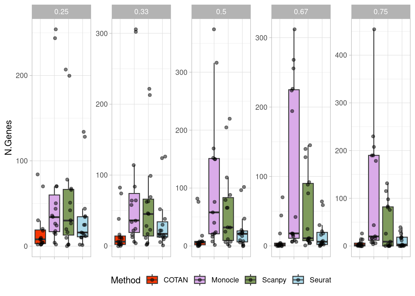
sessionInfo()R version 4.5.2 (2025-10-31)
Platform: x86_64-pc-linux-gnu
Running under: Ubuntu 22.04.5 LTS
Matrix products: default
BLAS: /usr/lib/x86_64-linux-gnu/blas/libblas.so.3.10.0
LAPACK: /usr/lib/x86_64-linux-gnu/lapack/liblapack.so.3.10.0 LAPACK version 3.10.0
locale:
[1] LC_CTYPE=C.UTF-8 LC_NUMERIC=C LC_TIME=C.UTF-8
[4] LC_COLLATE=C.UTF-8 LC_MONETARY=C.UTF-8 LC_MESSAGES=C.UTF-8
[7] LC_PAPER=C.UTF-8 LC_NAME=C LC_ADDRESS=C
[10] LC_TELEPHONE=C LC_MEASUREMENT=C.UTF-8 LC_IDENTIFICATION=C
time zone: Europe/Rome
tzcode source: system (glibc)
attached base packages:
[1] stats4 stats graphics grDevices utils datasets methods
[8] base
other attached packages:
[1] viridis_0.6.5 viridisLite_0.4.2
[3] ggplot2_4.0.1 tidyr_1.3.1
[5] dplyr_1.1.4 stringr_1.6.0
[7] reticulate_1.44.1 monocle3_1.3.7
[9] SingleCellExperiment_1.32.0 SummarizedExperiment_1.38.1
[11] GenomicRanges_1.62.1 Seqinfo_1.0.0
[13] IRanges_2.44.0 S4Vectors_0.48.0
[15] MatrixGenerics_1.22.0 matrixStats_1.5.0
[17] Biobase_2.70.0 BiocGenerics_0.56.0
[19] generics_0.1.3 Seurat_5.4.0
[21] SeuratObject_5.3.0 sp_2.2-0
[23] COTAN_2.11.1
loaded via a namespace (and not attached):
[1] RcppAnnoy_0.0.22 splines_4.5.2 later_1.4.2
[4] tibble_3.3.0 polyclip_1.10-7 fastDummies_1.7.5
[7] lifecycle_1.0.4 Rdpack_2.6.4 doParallel_1.0.17
[10] globals_0.18.0 lattice_0.22-7 MASS_7.3-65
[13] ggdist_3.3.3 dendextend_1.19.0 magrittr_2.0.4
[16] plotly_4.11.0 rmarkdown_2.29 yaml_2.3.10
[19] httpuv_1.6.16 otel_0.2.0 sctransform_0.4.2
[22] spam_2.11-1 spatstat.sparse_3.1-0 minqa_1.2.8
[25] cowplot_1.2.0 pbapply_1.7-2 RColorBrewer_1.1-3
[28] abind_1.4-8 Rtsne_0.17 purrr_1.2.0
[31] circlize_0.4.16 GenomeInfoDbData_1.2.14 ggrepel_0.9.6
[34] irlba_2.3.5.1 listenv_0.10.0 spatstat.utils_3.2-1
[37] goftest_1.2-3 RSpectra_0.16-2 spatstat.random_3.4-3
[40] fitdistrplus_1.2-2 parallelly_1.46.0 codetools_0.2-20
[43] DelayedArray_0.36.0 tidyselect_1.2.1 shape_1.4.6.1
[46] UCSC.utils_1.4.0 farver_2.1.2 lme4_1.1-37
[49] ScaledMatrix_1.16.0 spatstat.explore_3.6-0 jsonlite_2.0.0
[52] GetoptLong_1.1.0 progressr_0.18.0 ggridges_0.5.6
[55] survival_3.8-3 iterators_1.0.14 foreach_1.5.2
[58] tools_4.5.2 ica_1.0-3 Rcpp_1.1.0
[61] glue_1.8.0 gridExtra_2.3 SparseArray_1.10.8
[64] xfun_0.52 distributional_0.6.0 ggthemes_5.2.0
[67] GenomeInfoDb_1.44.0 withr_3.0.2 fastmap_1.2.0
[70] boot_1.3-32 digest_0.6.37 rsvd_1.0.5
[73] parallelDist_0.2.6 R6_2.6.1 mime_0.13
[76] colorspace_2.1-1 scattermore_1.2 tensor_1.5
[79] spatstat.data_3.1-9 data.table_1.18.0 httr_1.4.7
[82] htmlwidgets_1.6.4 S4Arrays_1.10.1 uwot_0.2.3
[85] pkgconfig_2.0.3 gtable_0.3.6 ComplexHeatmap_2.26.0
[88] lmtest_0.9-40 S7_0.2.1 XVector_0.50.0
[91] htmltools_0.5.8.1 dotCall64_1.2 zigg_0.0.2
[94] clue_0.3-66 scales_1.4.0 png_0.1-8
[97] reformulas_0.4.1 spatstat.univar_3.1-6 knitr_1.50
[100] reshape2_1.4.4 rjson_0.2.23 nloptr_2.2.1
[103] nlme_3.1-168 proxy_0.4-29 zoo_1.8-14
[106] GlobalOptions_0.1.2 KernSmooth_2.23-26 parallel_4.5.2
[109] miniUI_0.1.2 pillar_1.11.1 grid_4.5.2
[112] vctrs_0.7.0 RANN_2.6.2 promises_1.5.0
[115] BiocSingular_1.26.1 beachmat_2.26.0 xtable_1.8-4
[118] cluster_2.1.8.1 evaluate_1.0.5 zeallot_0.2.0
[121] cli_3.6.5 compiler_4.5.2 rlang_1.1.7
[124] crayon_1.5.3 future.apply_1.20.0 plyr_1.8.9
[127] stringi_1.8.7 deldir_2.0-4 BiocParallel_1.44.0
[130] assertthat_0.2.1 lazyeval_0.2.2 spatstat.geom_3.6-1
[133] Matrix_1.7-4 RcppHNSW_0.6.0 patchwork_1.3.2
[136] future_1.69.0 shiny_1.12.1 rbibutils_2.3
[139] ROCR_1.0-11 Rfast_2.1.5.1 igraph_2.2.1
[142] RcppParallel_5.1.10