library(COTAN)
library(ComplexHeatmap)
library(circlize)
library(dplyr)
library(Hmisc)
library(Seurat)
library(patchwork)
library(Rfast)
library(parallel)
library(doParallel)
library(HiClimR)
library(stringr)
library(fst)

options(parallelly.fork.enable = TRUE)

dataSetFile <- "Data/MouseCortex/MouseCortex_E14.5.cotan.RDS"
name <- str_split(dataSetFile,pattern = "/",simplify = T)[3]
name <- str_remove(name,pattern = ".RDS")

project = "E14.5"


setLoggingLevel(1)
outDir <- "CoexData/"
setLoggingFile(paste0(outDir, "Logs/",name,".log"))

obj <- readRDS(dataSetFile)
file_code = getMetadataElement(obj, datasetTags()[["cond"]])Gene Correlation Analysis E14.5 Mouse Cortex
Prologue
source("src/Functions.R")To compare the ability of COTAN to asses the real correlation between genes we define some pools of genes:
- Constitutive genes
- Neural progenitor genes
- Pan neuronal genes
- Some layer marker genes
genesList <- list(
  "NPGs"=
    c("Nes", "Vim", "Sox2", "Sox1", "Notch1", "Hes1", "Hes5", "Pax6"),
  "PNGs"=
    c("Map2", "Tubb3", "Neurod1", "Nefm", "Nefl", "Dcx", "Tbr1"),
  "hk"=
    c("Calm1", "Cox6b1", "Ppia", "Rpl18", "Cox7c", "Erh", "H3f3a",
      "Taf1", "Taf2", "Gapdh", "Actb", "Golph3", "Zfr", "Sub1",
      "Tars", "Amacr"),
  "layers" =
    c("Reln","Lhx5","Cux1","Satb2","Tle1","Mef2c","Rorb","Sox5","Bcl11b","Fezf2","Foxp2","Ntf3","Rasgrf2","Pvrl3", "Cux2","Slc17a6", "Sema3c","Thsd7a", "Sulf2", "Kcnk2","Grik3", "Etv1", "Tle4", "Tmem200a", "Glra2", "Etv1","Htr1f", "Sulf1","Rxfp1", "Syt6")
  # From https://www.science.org/doi/10.1126/science.aam8999
)
COTAN
genesFromListExpressed <- unlist(genesList)[unlist(genesList) %in% getGenes(obj)]
int.genes <-getGenes(obj)
coexMat.big <- getGenesCoex(obj)[genesFromListExpressed,genesFromListExpressed]
coexMat <- getGenesCoex(obj)[c(genesList$NPGs,genesList$hk,genesList$PNGs),c(genesList$NPGs,genesList$hk,genesList$PNGs)]
f1 = colorRamp2(seq(-0.5,0.5, length = 3), c("#DC0000B2", "white","#3C5488B2" ))
split.genes <- base::factor(c(rep("NPGs",length(genesList[["NPGs"]])),
rep("HK",length(genesList[["hk"]])),
rep("PNGs",length(genesList[["PNGs"]]))
),
levels = c("NPGs","HK","PNGs"))
lgd = Legend(col_fun = f1, title = "COTAN coex")
htmp <- Heatmap(as.matrix(coexMat),
#width = ncol(coexMat)*unit(2.5, "mm"),
height = nrow(coexMat)*unit(3, "mm"),
cluster_rows = FALSE,
cluster_columns = FALSE,
col = f1,
row_names_side = "left",
row_names_gp = gpar(fontsize = 11),
column_names_gp = gpar(fontsize = 11),
column_split = split.genes,
row_split = split.genes,
cluster_row_slices = FALSE,
cluster_column_slices = FALSE,
heatmap_legend_param = list(
title = "COTAN coex", at = c(-0.5, 0, 0.5),
direction = "horizontal",
labels = c("-0.5", "0", "0.5")
)
)
draw(htmp, heatmap_legend_side="right")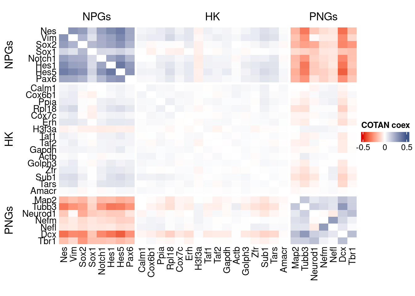
GDI_DF <- calculateGDI(obj)
GDI_DF$geneType <- NA
for (cat in names(genesList)) {
  GDI_DF[rownames(GDI_DF) %in% genesList[[cat]],]$geneType <- cat
}

GDI_DF$GDI_centered <- scale(GDI_DF$GDI,center = T,scale = T)

GDI_DF[genesFromListExpressed,]
sum.raw.norm GDI exp.cells geneType GDI_centered
Nes 8.839957 4.678500 27.7337997 NPGs 3.63695691
Vim 10.246463 4.534465 51.0309278 NPGs 3.42694609
Sox2 9.124228 4.566666 31.4709131 NPGs 3.47389659
Sox1 7.368458 3.455731 9.5636966 NPGs 1.85409012
Notch1 7.469284 4.355698 11.6623711 NPGs 3.16629269
Hes1 7.698079 4.634264 10.5946244 NPGs 3.57245806
Hes5 9.405265 4.812530 22.7908689 NPGs 3.83238101
Pax6 8.144613 4.367938 17.3877025 NPGs 3.18413945
Map2 10.172685 3.768818 72.7172312 PNGs 2.31058907
Tubb3 11.537925 4.586213 88.3836524 PNGs 3.50239807
Neurod1 8.881391 3.388955 22.9657585 PNGs 1.75672703
Nefm 8.288330 3.346732 17.5441826 PNGs 1.69516332
Nefl 7.678477 3.544436 8.6340206 PNGs 1.98342736
Dcx 10.120356 4.821636 66.9090574 PNGs 3.84565720
Tbr1 8.472723 3.926272 24.1715758 PNGs 2.54016525
Calm1 11.491577 1.857652 96.5114138 hk -0.47600225
Cox6b1 10.398257 1.992891 84.6833579 hk -0.27881530
Ppia 7.666735 2.386108 17.4797496 hk 0.29451755
Rpl18 9.176712 2.575898 51.5187776 hk 0.57124278
Cox7c 8.439961 1.902976 31.8206922 hk -0.40991709
Erh 6.593118 2.307720 6.5721649 hk 0.18022355
H3f3a 9.388420 1.886267 58.1093520 hk -0.43428010
Taf1 8.315368 2.138643 26.8869661 hk -0.06630076
Taf2 8.017975 1.861938 21.1432253 hk -0.46975224
Gapdh 5.018736 1.853094 1.5648012 hk -0.48264772
Actb 12.609181 1.492016 99.6778351 hk -1.00911996
Golph3 7.150183 1.851371 10.8891753 hk -0.48515921
Zfr 9.269238 2.273001 50.7916053 hk 0.12960056
Sub1 10.018254 2.583820 74.7238586 hk 0.58279347
Tars 8.056910 2.487556 22.8645066 hk 0.44243393
Amacr 5.492910 1.714319 2.2551546 hk -0.68499008
Reln 7.095360 3.011725 4.5563328 layers 1.20670295
Lhx5 6.037778 2.901306 2.0434462 layers 1.04570542
Cux1 8.597262 3.026589 31.3512518 layers 1.22837610
Satb2 7.603191 3.121471 11.0916789 layers 1.36671855
Tle1 7.891909 2.322600 17.8111193 layers 0.20191897
Mef2c 8.776162 4.057560 23.6377025 layers 2.73159053
Rorb 6.523092 1.943768 4.6023564 layers -0.35043950
Sox5 9.301863 3.584350 38.2639912 layers 2.04162343
Bcl11b 9.860621 4.189936 53.4057437 layers 2.92460213
Fezf2 8.804060 3.630239 28.8751841 layers 2.10853283
Foxp2 7.474618 2.254280 8.4867452 layers 0.10230519
Ntf3 4.673267 2.314479 0.8560383 layers 0.19007802
Pvrl3 7.255727 3.417288 10.6866716 layers 1.79803751
Cux2 7.652690 3.088322 11.2573638 layers 1.31838644
Slc17a6 7.901396 2.998305 14.0648012 layers 1.18713575
Sema3c 7.222013 2.481806 7.6307069 layers 0.43405122
Thsd7a 7.472372 3.054089 8.0449190 layers 1.26847311
Sulf2 6.491056 2.379550 4.6759941 layers 0.28495572
Kcnk2 7.151877 1.901258 9.0390280 layers -0.41242163
Grik3 6.673233 2.781234 5.3019146 layers 0.87063375
Etv1 6.743118 2.264998 4.8232695 layers 0.11793173
Tle4 7.880978 2.635418 15.0405007 layers 0.65802538
Tmem200a 6.188517 2.926026 3.8751841 layers 1.08174899
Glra2 7.057638 3.858495 8.1369661 layers 2.44134235
Etv1.1 6.743118 2.264998 4.8232695 layers 0.11793173
Sulf1 5.465717 2.461515 1.0125184 layers 0.40446505
Syt6 7.555334 3.052113 8.8457290 layers 1.26559064GDIPlot(obj,GDIIn = GDI_DF, genes = genesList,GDIThreshold = 1.4)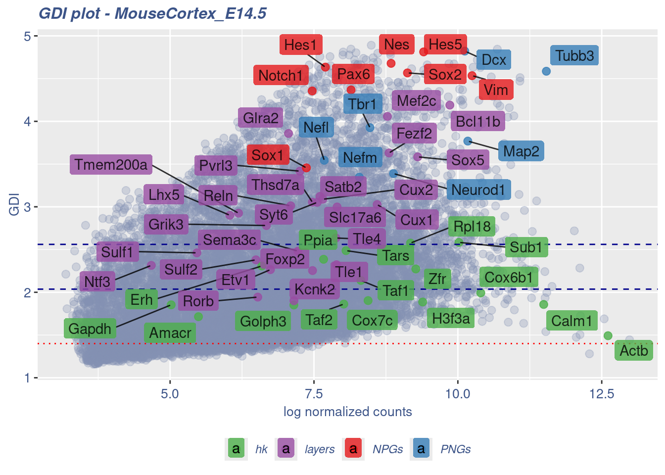
Seurat correlation
srat<- CreateSeuratObject(counts = getRawData(obj),
                          project = project,
                          min.cells = 3,
                          min.features = 200)
srat[["percent.mt"]] <- PercentageFeatureSet(srat, pattern = "^mt-")
srat <- NormalizeData(srat)
srat <- FindVariableFeatures(srat, selection.method = "vst", nfeatures = 2000)

# plot variable features with and without labels
plot1 <- VariableFeaturePlot(srat)

plot1$data$centered_variance <- scale(plot1$data$variance.standardized,
                                      center = T,scale = F)

write.csv(plot1$data,paste0("CoexData/",
                            "Variance_Seurat_genes",
                            getMetadataElement(obj,
                                               datasetTags()[["cond"]]),".csv"))

LabelPoints(plot = plot1, points = c(genesList$NPGs,genesList$PNGs,genesList$layers), repel = TRUE)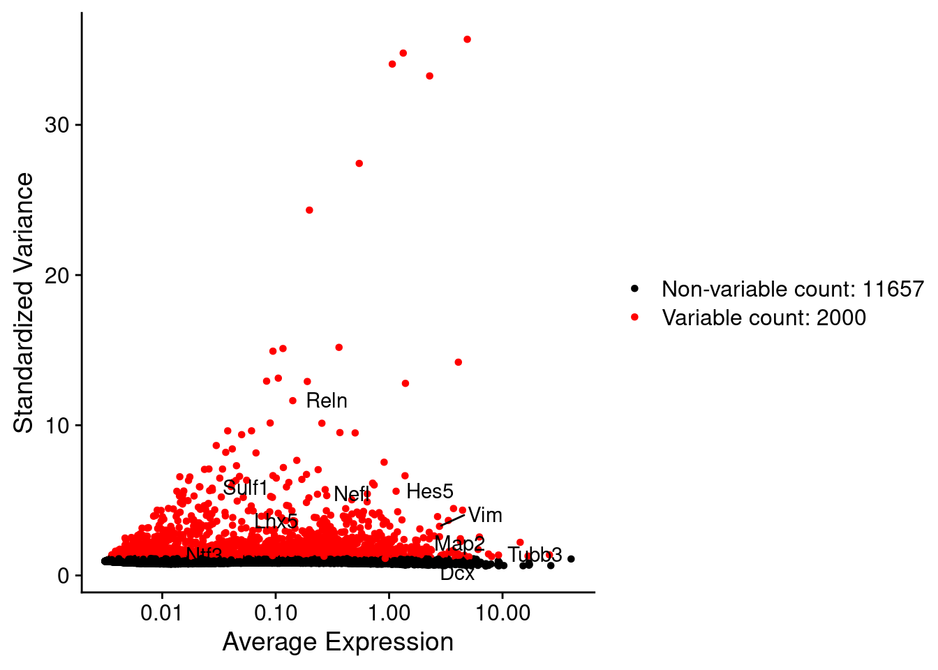
LabelPoints(plot = plot1, points = c(genesList$hk), repel = TRUE)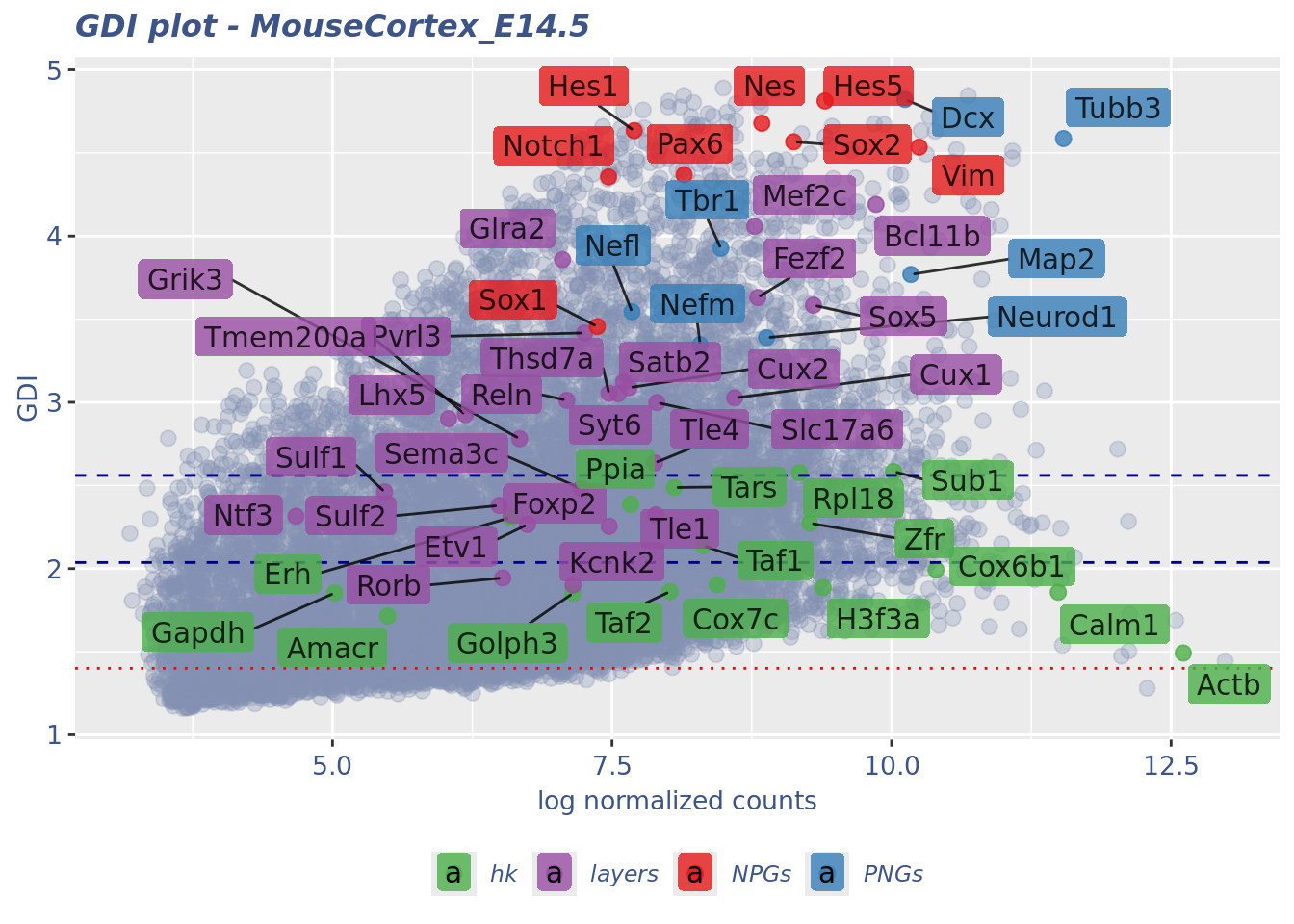
all.genes <- rownames(srat)
srat <- ScaleData(srat, features = all.genes)
seurat.data = GetAssayData(srat[["RNA"]],layer = "data")
corr.pval.list <- correlation_pvalues(data = seurat.data,
genesFromListExpressed,
n.cells = getNumCells(obj))
seurat.data.cor.big <- as.matrix(Matrix::forceSymmetric(corr.pval.list$data.cor, uplo = "U"))
htmp <- correlation_plot(seurat.data.cor.big,
genesList, title="Seurat corr")
p_values.fromSeurat <- corr.pval.list$p_values
seurat.data.cor.big <- corr.pval.list$data.cor
rm(corr.pval.list)
gc() used (Mb) gc trigger (Mb) max used (Mb)
Ncells 10156112 542.4 17749498 948.0 17749498 948.0
Vcells 386493768 2948.8 717720243 5475.8 740876735 5652.5draw(htmp, heatmap_legend_side="right")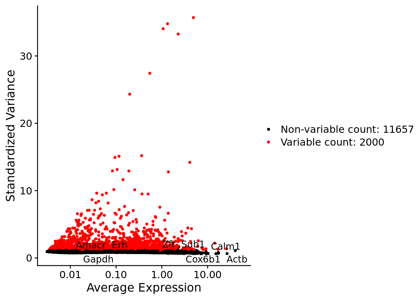
rm(seurat.data.cor.big)
rm(p_values.fromSeurat)
Seurat SC Transform
srat <-  SCTransform(srat,
                     method = "glmGamPoi",
                     vars.to.regress = "percent.mt",
                     verbose = FALSE)

seurat.data <- GetAssayData(srat[["SCT"]],layer = "data")

#Remove genes with all zeros
seurat.data <-seurat.data[rowSums(seurat.data) > 0,]


corr.pval.list <- correlation_pvalues(seurat.data,
                                      genesFromListExpressed,
                                      n.cells = getNumCells(obj))


seurat.data.cor.big <- as.matrix(Matrix::forceSymmetric(corr.pval.list$data.cor, uplo = "U"))

htmp <- correlation_plot(seurat.data.cor.big,
                         genesList, title="Seurat corr SCT")


p_values.fromSeurat <- corr.pval.list$p_values
seurat.data.cor.big <- corr.pval.list$data.cor

rm(corr.pval.list)
gc()
used (Mb) gc trigger (Mb) max used (Mb)
Ncells 10484557 560.0 17749498 948.0 17749498 948.0
Vcells 474103212 3617.2 1240511778 9464.4 1240500358 9464.3draw(htmp, heatmap_legend_side="right")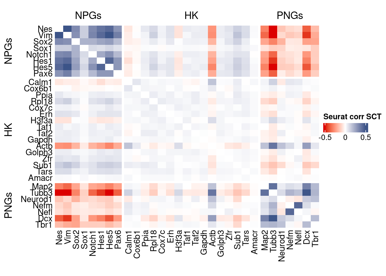
plot1 <- VariableFeaturePlot(srat)

plot1$data$centered_variance <- scale(plot1$data$residual_variance,
center = T,scale = F)write.csv(plot1$data,paste0("CoexData/",
"Variance_SeuratSCT_genes",
getMetadataElement(obj,
datasetTags()[["cond"]]),".csv"))
write_fst(as.data.frame(seurat.data.cor.big),path = paste0("CoexData/SeuratCorrSCT_",file_code,".fst"), compress = 100)
write_fst(as.data.frame(p_values.fromSeurat),path = paste0("CoexData/SeuratPValuesSCT_", file_code,".fst"))
write.csv(as.data.frame(p_values.fromSeurat),paste0("CoexData/SeuratPValuesSCT_", file_code,".csv"))
rm(seurat.data.cor.big)
rm(p_values.fromSeurat)Monocle
library(monocle3)cds <- new_cell_data_set(getRawData(obj),
cell_metadata = getMetadataCells(obj),
gene_metadata = getMetadataGenes(obj)
)
cds <- preprocess_cds(cds, num_dim = 100)
normalized_counts <- normalized_counts(cds)#Remove genes with all zeros
normalized_counts <- normalized_counts[rowSums(normalized_counts) > 0,]
corr.pval.list <- correlation_pvalues(normalized_counts,
genesFromListExpressed,
n.cells = getNumCells(obj))
rm(normalized_counts)
monocle.data.cor.big <- as.matrix(Matrix::forceSymmetric(corr.pval.list$data.cor, uplo = "U"))
htmp <- correlation_plot(data.cor.big = monocle.data.cor.big,
genesList,
title = "Monocle corr")
p_values.from.monocle <- corr.pval.list$p_values
monocle.data.cor.big <- corr.pval.list$data.cor
rm(corr.pval.list)
gc() used (Mb) gc trigger (Mb) max used (Mb)
Ncells 10670810 569.9 17749498 948.0 17749498 948.0
Vcells 476917692 3638.6 1240511778 9464.4 1240500358 9464.3draw(htmp, heatmap_legend_side="right")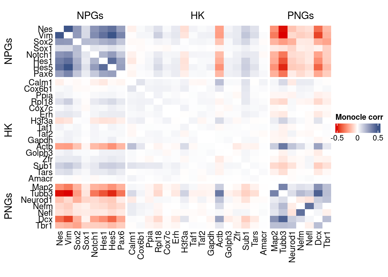
Cs-Core
library(CSCORE)Convert to Seurat obj
sceObj <- convertToSingleCellExperiment(obj)

# Correct: assay=NULL (or omit), data=NULL (since no logcounts)
seuratObj <- as.Seurat(
  x       = sceObj,
  counts  = "counts",
  data    = NULL,
  assay   = NULL,      # IMPORTANT: do NOT set to "RNA" here
  project = "COTAN"
)

# as.Seurat(SCE) creates assay "originalexp" by default; rename it to RNA
seuratObj <- RenameAssays(seuratObj, originalexp = "RNA", verbose = FALSE)
DefaultAssay(seuratObj) <- "RNA"

# Optional: keep COTAN payload
seuratObj@misc$COTAN <- S4Vectors::metadata(sceObj)
Extract CS_CORE corr matrix
#seuratObj@assays$RNA@counts <- ceiling(seuratObj@assays$RNA@counts)
csCoreRes <- CSCORE(seuratObj, genes = genesFromListExpressed)
[INFO] IRLS converged after 3 iterations.
[INFO] Starting WLS for covariance at Wed Jan 21 11:27:26 2026
[INFO] 1 among 58 genes have invalid variance estimates. Their co-expressions with other genes were set to 0.
[INFO] 0.0605% co-expression estimates were greater than 1 and were set to 1.
[INFO] 0.0000% co-expression estimates were smaller than -1 and were set to -1.
[INFO] Finished WLS. Elapsed time: 0.3003 seconds.mat <- as.matrix(csCoreRes$est)
diag(mat) <- 0
split.genes <- base::factor(c(rep("NPGs",sum(genesList[["NPGs"]] %in% genesFromListExpressed)),
rep("HK",sum(genesList[["hk"]] %in% genesFromListExpressed)),
rep("PNGs",sum(genesList[["PNGs"]] %in% genesFromListExpressed))
),
levels = c("NPGs","HK","PNGs"))
f1 = colorRamp2(seq(-0.5,0.5, length = 3), c("#DC0000B2", "white","#3C5488B2" ))
htmp <- Heatmap(as.matrix(mat[c(genesList$NPGs,genesList$hk,genesList$PNGs),c(genesList$NPGs,genesList$hk,genesList$PNGs)]),
#width = ncol(coexMat)*unit(2.5, "mm"),
height = nrow(mat)*unit(3, "mm"),
cluster_rows = FALSE,
cluster_columns = FALSE,
col = f1,
row_names_side = "left",
row_names_gp = gpar(fontsize = 11),
column_names_gp = gpar(fontsize = 11),
column_split = split.genes,
row_split = split.genes,
cluster_row_slices = FALSE,
cluster_column_slices = FALSE,
heatmap_legend_param = list(
title = "CS-CORE", at = c(-0.5, 0, 0.5),
direction = "horizontal",
labels = c("-0.5", "0", "0.5")
)
)
draw(htmp, heatmap_legend_side="right")
Save CS_CORE matrix
write_fst(as.data.frame(csCoreRes$est), path = paste0("CoexData/CS_CORECorr_", file_code,".fst"),compress = 100)
write_fst(as.data.frame(csCoreRes$p_value), path = paste0("CoexData/CS_COREPValues_", file_code,".fst"),compress = 100)
write.csv(as.data.frame(csCoreRes$p_value), paste0("CoexData/CS_COREPValues_", file_code,".csv"))
Baseline: Spearman on UMI counts
corr.pval.list <- correlation_pvaluesSpearman(data = getRawData(obj),
                                      genesFromListExpressed,
                                      n.cells = getNumCells(obj))

data.cor.big <- as.matrix(Matrix::forceSymmetric(corr.pval.list$data.cor, uplo = "U"))

htmp <- correlation_plot(data.cor.big,
                         genesList, title="UMI baseline S. corr")


p_values.fromSp.C <- corr.pval.list$p_values
data.cor.bigSp.C <- corr.pval.list$data.cor

rm(corr.pval.list)
gc()
used (Mb) gc trigger (Mb) max used (Mb)
Ncells 10679205 570.4 17749498 948.0 17749498 948.0
Vcells 477099407 3640.0 1240511778 9464.4 1240500358 9464.3draw(htmp, heatmap_legend_side="right")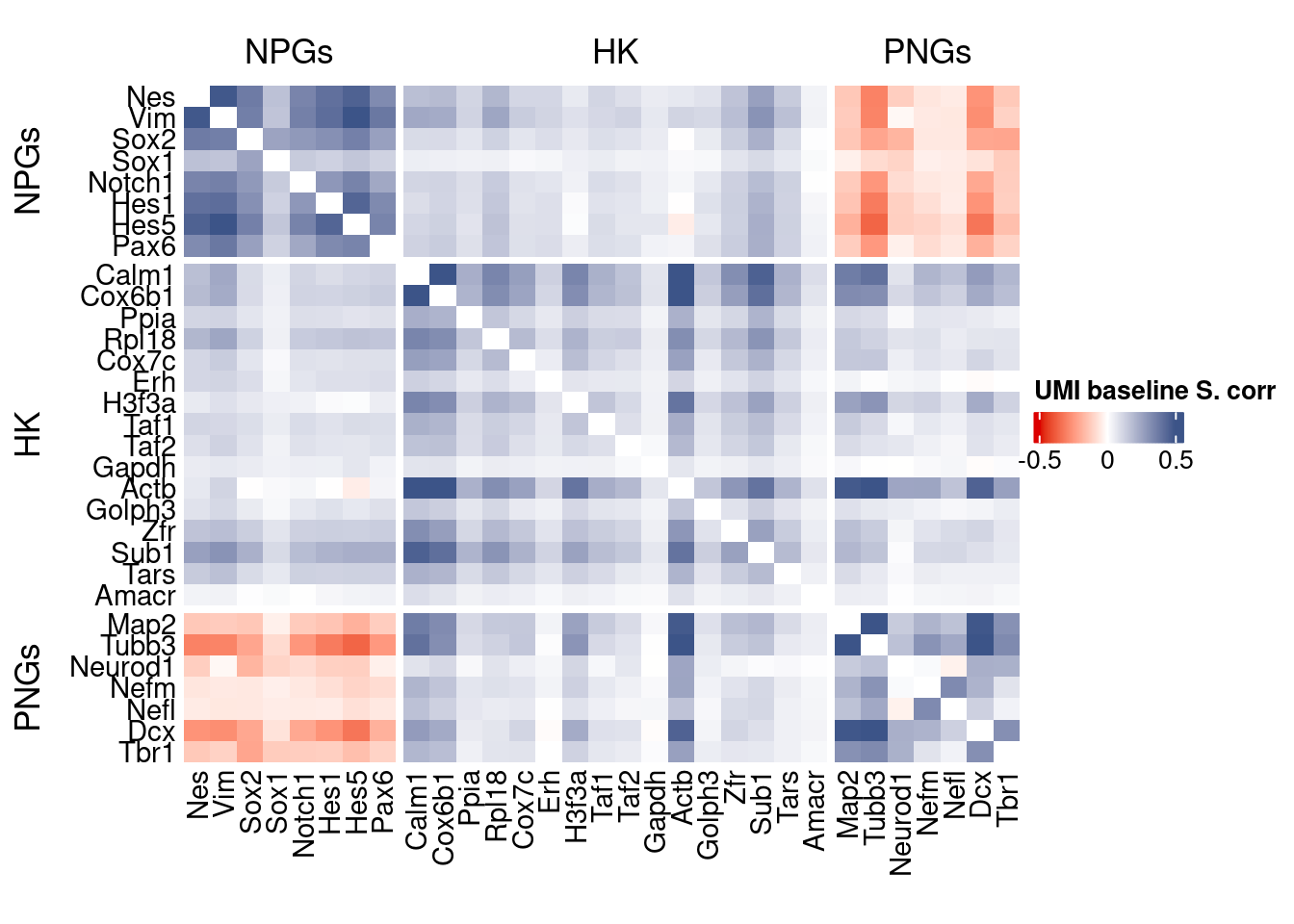
write.csv(as.data.frame(p_values.fromSp.C), paste0("CoexData/BaselineUMISpCorrPValues_", file_code,".csv"))Baseline: Pearson on binarized counts
corr.pval.list <- correlation_pvalues(data = getZeroOneProj(obj),
                                      genesFromListExpressed,
                                      n.cells = getNumCells(obj))

data.cor.big <- as.matrix(Matrix::forceSymmetric(corr.pval.list$data.cor, uplo = "U"))

htmp <- correlation_plot(data.cor.big,
                         genesList, title="Zero-one P. corr")


p_values.fromSp.C <- corr.pval.list$p_values
data.cor.bigSp.C <- corr.pval.list$data.cor

rm(corr.pval.list)
gc()
used (Mb) gc trigger (Mb) max used (Mb)
Ncells 10679332 570.4 17749498 948.0 17749498 948.0
Vcells 477099664 3640.0 1240511778 9464.4 1240500358 9464.3draw(htmp, heatmap_legend_side="right")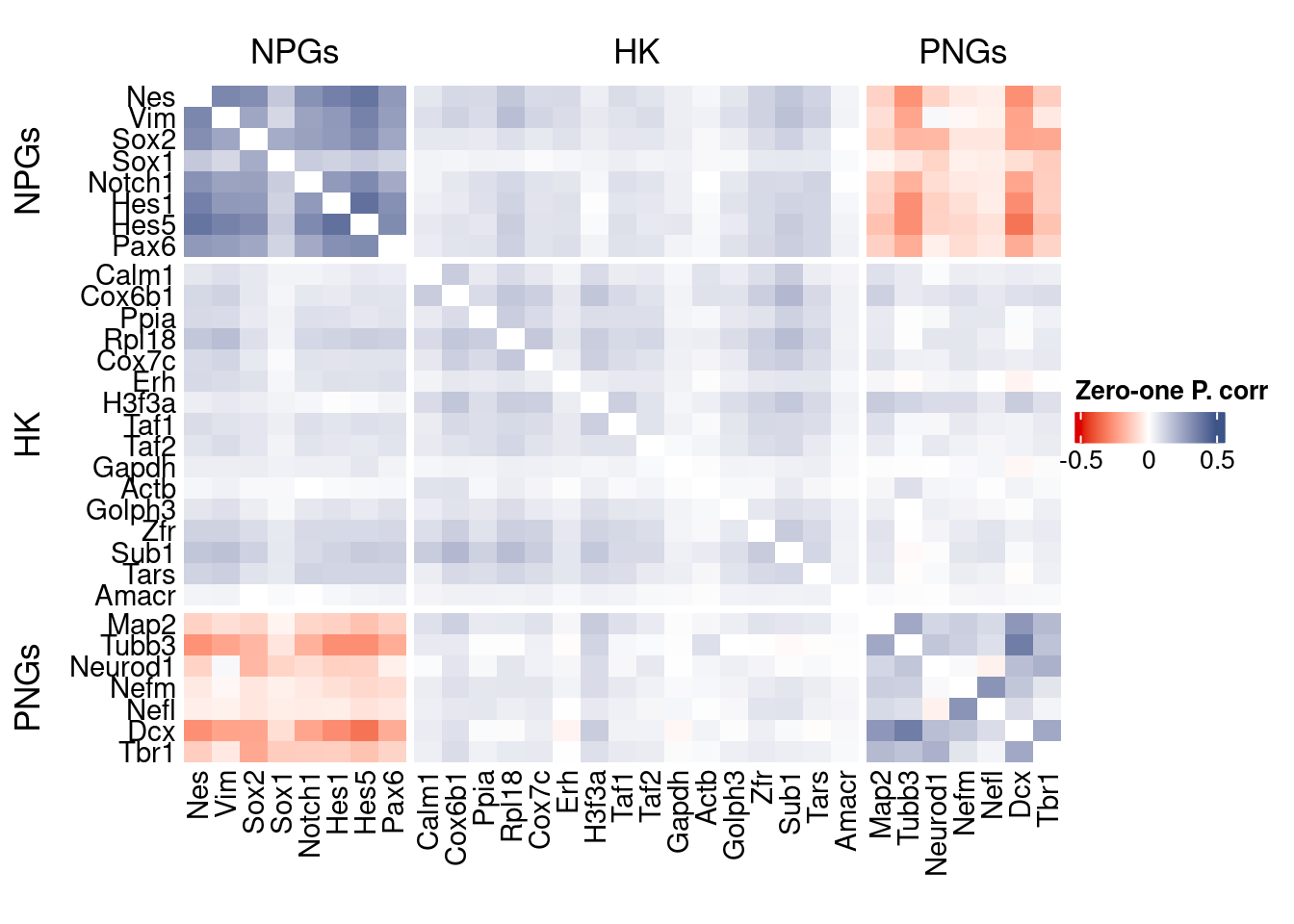
write.csv(as.data.frame(p_values.fromSp.C), paste0("CoexData/ZeroOnePCorrPValues_", file_code,".csv"))Sys.time()[1] "2026-01-21 11:27:31 CET"sessionInfo()R version 4.5.2 (2025-10-31)
Platform: x86_64-pc-linux-gnu
Running under: Ubuntu 22.04.5 LTS
Matrix products: default
BLAS: /usr/lib/x86_64-linux-gnu/blas/libblas.so.3.10.0
LAPACK: /usr/lib/x86_64-linux-gnu/lapack/liblapack.so.3.10.0 LAPACK version 3.10.0
locale:
[1] LC_CTYPE=C.UTF-8 LC_NUMERIC=C LC_TIME=C.UTF-8
[4] LC_COLLATE=C.UTF-8 LC_MONETARY=C.UTF-8 LC_MESSAGES=C.UTF-8
[7] LC_PAPER=C.UTF-8 LC_NAME=C LC_ADDRESS=C
[10] LC_TELEPHONE=C LC_MEASUREMENT=C.UTF-8 LC_IDENTIFICATION=C
time zone: Europe/Rome
tzcode source: system (glibc)
attached base packages:
[1] stats4 parallel grid stats graphics grDevices utils
[8] datasets methods base
other attached packages:
[1] CSCORE_1.0.2 monocle3_1.3.7
[3] SingleCellExperiment_1.32.0 SummarizedExperiment_1.38.1
[5] GenomicRanges_1.62.1 Seqinfo_1.0.0
[7] IRanges_2.44.0 S4Vectors_0.48.0
[9] MatrixGenerics_1.22.0 matrixStats_1.5.0
[11] Biobase_2.70.0 BiocGenerics_0.56.0
[13] generics_0.1.3 fstcore_0.10.0
[15] fst_0.9.8 stringr_1.6.0
[17] HiClimR_2.2.1 doParallel_1.0.17
[19] iterators_1.0.14 foreach_1.5.2
[21] Rfast_2.1.5.1 RcppParallel_5.1.10
[23] zigg_0.0.2 Rcpp_1.1.0
[25] patchwork_1.3.2 Seurat_5.4.0
[27] SeuratObject_5.3.0 sp_2.2-0
[29] Hmisc_5.2-3 dplyr_1.1.4
[31] circlize_0.4.16 ComplexHeatmap_2.26.0
[33] COTAN_2.11.1
loaded via a namespace (and not attached):
[1] RcppAnnoy_0.0.22 splines_4.5.2
[3] later_1.4.2 tibble_3.3.0
[5] polyclip_1.10-7 rpart_4.1.24
[7] fastDummies_1.7.5 lifecycle_1.0.4
[9] Rdpack_2.6.4 globals_0.18.0
[11] lattice_0.22-7 MASS_7.3-65
[13] backports_1.5.0 ggdist_3.3.3
[15] dendextend_1.19.0 magrittr_2.0.4
[17] plotly_4.11.0 rmarkdown_2.29
[19] yaml_2.3.10 httpuv_1.6.16
[21] otel_0.2.0 glmGamPoi_1.20.0
[23] sctransform_0.4.2 spam_2.11-1
[25] spatstat.sparse_3.1-0 reticulate_1.44.1
[27] minqa_1.2.8 cowplot_1.2.0
[29] pbapply_1.7-2 RColorBrewer_1.1-3
[31] abind_1.4-8 Rtsne_0.17
[33] purrr_1.2.0 nnet_7.3-20
[35] GenomeInfoDbData_1.2.14 ggrepel_0.9.6
[37] irlba_2.3.5.1 listenv_0.10.0
[39] spatstat.utils_3.2-1 goftest_1.2-3
[41] RSpectra_0.16-2 spatstat.random_3.4-3
[43] fitdistrplus_1.2-2 parallelly_1.46.0
[45] DelayedMatrixStats_1.30.0 ncdf4_1.24
[47] codetools_0.2-20 DelayedArray_0.36.0
[49] tidyselect_1.2.1 shape_1.4.6.1
[51] UCSC.utils_1.4.0 farver_2.1.2
[53] lme4_1.1-37 ScaledMatrix_1.16.0
[55] viridis_0.6.5 base64enc_0.1-3
[57] spatstat.explore_3.6-0 jsonlite_2.0.0
[59] GetoptLong_1.1.0 Formula_1.2-5
[61] progressr_0.18.0 ggridges_0.5.6
[63] survival_3.8-3 tools_4.5.2
[65] ica_1.0-3 glue_1.8.0
[67] gridExtra_2.3 SparseArray_1.10.8
[69] xfun_0.52 distributional_0.6.0
[71] ggthemes_5.2.0 GenomeInfoDb_1.44.0
[73] withr_3.0.2 fastmap_1.2.0
[75] boot_1.3-32 digest_0.6.37
[77] rsvd_1.0.5 parallelDist_0.2.6
[79] R6_2.6.1 mime_0.13
[81] colorspace_2.1-1 Cairo_1.7-0
[83] scattermore_1.2 tensor_1.5
[85] spatstat.data_3.1-9 tidyr_1.3.1
[87] data.table_1.18.0 httr_1.4.7
[89] htmlwidgets_1.6.4 S4Arrays_1.10.1
[91] uwot_0.2.3 pkgconfig_2.0.3
[93] gtable_0.3.6 lmtest_0.9-40
[95] S7_0.2.1 XVector_0.50.0
[97] htmltools_0.5.8.1 dotCall64_1.2
[99] clue_0.3-66 scales_1.4.0
[101] png_0.1-8 reformulas_0.4.1
[103] spatstat.univar_3.1-6 rstudioapi_0.18.0
[105] knitr_1.50 reshape2_1.4.4
[107] rjson_0.2.23 nloptr_2.2.1
[109] checkmate_2.3.2 nlme_3.1-168
[111] proxy_0.4-29 zoo_1.8-14
[113] GlobalOptions_0.1.2 KernSmooth_2.23-26
[115] miniUI_0.1.2 foreign_0.8-90
[117] pillar_1.11.1 vctrs_0.7.0
[119] RANN_2.6.2 promises_1.5.0
[121] BiocSingular_1.26.1 beachmat_2.26.0
[123] xtable_1.8-4 cluster_2.1.8.1
[125] htmlTable_2.4.3 evaluate_1.0.5
[127] magick_2.9.0 zeallot_0.2.0
[129] cli_3.6.5 compiler_4.5.2
[131] rlang_1.1.7 crayon_1.5.3
[133] future.apply_1.20.0 labeling_0.4.3
[135] plyr_1.8.9 stringi_1.8.7
[137] viridisLite_0.4.2 deldir_2.0-4
[139] BiocParallel_1.44.0 assertthat_0.2.1
[141] lazyeval_0.2.2 spatstat.geom_3.6-1
[143] Matrix_1.7-4 RcppHNSW_0.6.0
[145] sparseMatrixStats_1.20.0 future_1.69.0
[147] ggplot2_4.0.1 shiny_1.12.1
[149] rbibutils_2.3 ROCR_1.0-11
[151] igraph_2.2.1