library(COTAN)
library(ComplexHeatmap)
library(circlize)
library(dplyr)
library(Hmisc)
library(Seurat)
library(patchwork)
library(Rfast)
library(parallel)
library(doParallel)
library(HiClimR)
library(stringr)
library(fst)

options(parallelly.fork.enable = TRUE)

dataSetFile <- "Data/MouseCortexFromLoom/e15.0_ForebrainDorsal.cotan.RDS"
name <- str_split(dataSetFile,pattern = "/",simplify = T)[3]
name <- str_remove(name,pattern = ".RDS")

project = "E15.0"


setLoggingLevel(1)
outDir <- "CoexData/"
setLoggingFile(paste0(outDir, "Logs/",name,".log"))

obj <- readRDS(dataSetFile)
file_code = getMetadataElement(obj, datasetTags()[["cond"]])Gene Correlation Analysis E15.0 Mouse Brain
Prologue
source("src/Functions.R")To compare the ability of COTAN to asses the real correlation between genes we define some pools of genes:
- Constitutive genes
- Neural progenitor genes
- Pan neuronal genes
- Some layer marker genes
genesList <- list(
  "NPGs"=
    c("Nes", "Vim", "Sox2", "Sox1", "Notch1", "Hes1", "Hes5", "Pax6"),
  "PNGs"=
    c("Map2", "Tubb3", "Neurod1", "Nefm", "Nefl", "Dcx", "Tbr1"),
  "hk"=
    c("Calm1", "Cox6b1", "Ppia", "Rpl18", "Cox7c", "Erh", "H3f3a",
      "Taf1", "Taf2", "Gapdh", "Actb", "Golph3", "Zfr", "Sub1",
      "Tars", "Amacr"),
  "layers" =
    c("Reln","Lhx5","Cux1","Satb2","Tle1","Mef2c","Rorb","Sox5","Bcl11b","Fezf2","Foxp2","Ntf3","Rasgrf2","Pvrl3", "Cux2","Slc17a6", "Sema3c","Thsd7a", "Sulf2", "Kcnk2","Grik3", "Etv1", "Tle4", "Tmem200a", "Glra2", "Etv1","Htr1f", "Sulf1","Rxfp1", "Syt6")
  # From https://www.science.org/doi/10.1126/science.aam8999
)
COTAN
genesFromListExpressed <- unlist(genesList)[unlist(genesList) %in% getGenes(obj)]
int.genes <-getGenes(obj)
coexMat.big <- getGenesCoex(obj)[genesFromListExpressed,genesFromListExpressed]
coexMat <- getGenesCoex(obj)[c(genesList$NPGs,genesList$hk,genesList$PNGs),c(genesList$NPGs,genesList$hk,genesList$PNGs)]
f1 = colorRamp2(seq(-0.5,0.5, length = 3), c("#DC0000B2", "white","#3C5488B2" ))
split.genes <- base::factor(c(rep("NPGs",length(genesList[["NPGs"]])),
rep("HK",length(genesList[["hk"]])),
rep("PNGs",length(genesList[["PNGs"]]))
),
levels = c("NPGs","HK","PNGs"))
lgd = Legend(col_fun = f1, title = "COTAN coex")
htmp <- Heatmap(as.matrix(coexMat),
#width = ncol(coexMat)*unit(2.5, "mm"),
height = nrow(coexMat)*unit(3, "mm"),
cluster_rows = FALSE,
cluster_columns = FALSE,
col = f1,
row_names_side = "left",
row_names_gp = gpar(fontsize = 11),
column_names_gp = gpar(fontsize = 11),
column_split = split.genes,
row_split = split.genes,
cluster_row_slices = FALSE,
cluster_column_slices = FALSE,
heatmap_legend_param = list(
title = "COTAN coex", at = c(-0.5, 0, 0.5),
direction = "horizontal",
labels = c("-0.5", "0", "0.5")
)
)
draw(htmp, heatmap_legend_side="right")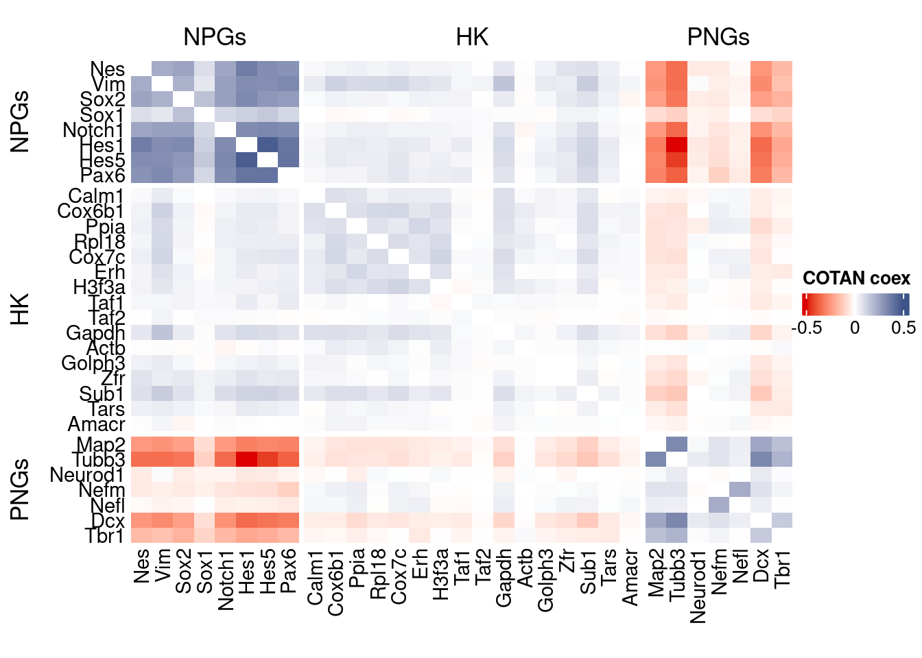
GDI_DF <- calculateGDI(obj)
GDI_DF$geneType <- NA
for (cat in names(genesList)) {
  GDI_DF[rownames(GDI_DF) %in% genesList[[cat]],]$geneType <- cat
}

GDI_DF$GDI_centered <- scale(GDI_DF$GDI,center = T,scale = T)

GDI_DF[genesFromListExpressed,]
sum.raw.norm GDI exp.cells geneType GDI_centered
Nes 7.036617 4.395412 10.3013315 NPGs 2.844118518
Vim 9.750744 4.622956 44.6274235 NPGs 3.141716247
Sox2 6.748800 4.388553 7.8019154 NPGs 2.835147083
Sox1 5.573231 2.954812 2.4760570 NPGs 0.959999758
Notch1 6.804377 4.507208 8.3158141 NPGs 2.990333393
Hes1 7.293684 5.025427 8.7362766 NPGs 3.668097091
Hes5 7.762615 4.779269 10.1845363 NPGs 3.346154337
Pax6 7.996731 4.881428 18.3368372 NPGs 3.479764633
Map2 10.179711 4.599886 82.3872927 PNGs 3.111544365
Tubb3 11.940548 5.083784 90.3527213 PNGs 3.744420459
Neurod1 5.831083 2.015123 3.2936230 PNGs -0.268991989
Nefm 6.753599 3.152181 7.2996963 PNGs 1.218132436
Nefl 6.160391 2.932141 2.9081990 PNGs 0.930349401
Dcx 9.308480 4.495594 58.9581873 PNGs 2.975143901
Tbr1 8.629160 3.877197 34.4662462 PNGs 2.166359967
Calm1 11.069821 2.194787 97.4421864 hk -0.034015260
Cox6b1 10.240794 2.951945 90.9950946 hk 0.956249628
Ppia 10.343824 2.955456 89.4183602 hk 0.960842148
Rpl18 10.858263 2.901626 96.6596590 hk 0.890439277
Cox7c 10.245556 3.030177 90.4578370 hk 1.058567954
Erh 9.288155 2.659736 65.1016118 hk 0.574079159
H3f3a 11.042683 2.850307 97.6991357 hk 0.823321315
Taf1 7.373313 1.751203 15.6855875 hk -0.614165195
Taf2 7.069134 1.415716 11.9247839 hk -1.052939358
Gapdh 10.083151 3.161859 85.3422098 hk 1.230790542
Actb 11.906861 1.608850 99.5912170 hk -0.800344008
Golph3 7.440459 1.866369 17.4842327 hk -0.463542657
Zfr 8.645382 2.219651 44.1485634 hk -0.001496122
Sub1 9.822502 3.217085 80.7171222 hk 1.303018400
Tars 7.476170 1.988439 17.9981313 hk -0.303891645
Amacr 5.810916 1.827868 3.9710348 hk -0.513897792
Reln 8.349205 2.819876 8.3625321 layers 0.783521463
Lhx5 5.830435 3.139114 1.8220042 layers 1.201042642
Cux1 8.606685 3.850086 34.5713618 layers 2.130902087
Satb2 9.146209 3.735391 31.3361364 layers 1.980896809
Tle1 8.069147 2.752489 25.8000467 layers 0.695387361
Mef2c 9.310240 4.395042 37.2226115 layers 2.843634817
Rorb 7.450810 2.392823 10.9437047 layers 0.224990367
Sox5 10.622002 4.093212 73.5926185 layers 2.448880218
Bcl11b 9.575893 4.600605 54.8937164 layers 3.112483916
Fezf2 9.378784 3.369265 51.6935295 layers 1.502050523
Foxp2 8.380413 3.553319 23.5342210 layers 1.742770215
Ntf3 5.324482 2.116601 1.8920813 layers -0.136271617
Cux2 7.592847 3.129196 12.2401308 layers 1.188071005
Slc17a6 7.647733 3.418696 13.7351086 layers 1.566700439
Sema3c 7.661987 2.896666 13.8752628 layers 0.883952732
Thsd7a 6.173797 2.313999 3.1067508 layers 0.121899301
Sulf2 5.738452 2.925339 2.7914039 layers 0.921453194
Kcnk2 8.245680 2.304727 27.1548704 layers 0.109773149
Grik3 7.243325 3.637511 10.5349217 layers 1.852881971
Etv1 6.019894 2.984098 3.2235459 layers 0.998302023
Tle4 7.432453 2.929052 13.0343378 layers 0.926308788
Tmem200a 6.201199 2.658151 4.7886008 layers 0.572005411
Glra2 7.633574 3.878564 13.7467881 layers 2.168147973
Etv1.1 6.019894 2.984098 3.2235459 layers 0.998302023
Htr1f 4.884079 2.283998 1.0394768 layers 0.082662331
Sulf1 4.901491 2.120374 0.7241299 layers -0.131337122
Syt6 6.394410 2.800827 4.5082925 layers 0.758607816GDIPlot(obj,GDIIn = GDI_DF, genes = genesList,GDIThreshold = 1.4)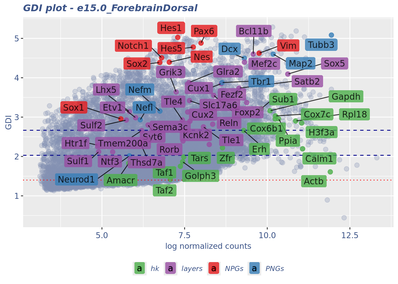
Seurat correlation
srat<- CreateSeuratObject(counts = getRawData(obj),
                          project = project,
                          min.cells = 3,
                          min.features = 200)
srat[["percent.mt"]] <- PercentageFeatureSet(srat, pattern = "^mt-")
srat <- NormalizeData(srat)
srat <- FindVariableFeatures(srat, selection.method = "vst", nfeatures = 2000)

# plot variable features with and without labels
plot1 <- VariableFeaturePlot(srat)

plot1$data$centered_variance <- scale(plot1$data$variance.standardized,
                                      center = T,scale = F)

write.csv(plot1$data,paste0("CoexData/",
                            "Variance_Seurat_genes",
                            getMetadataElement(obj,
                                               datasetTags()[["cond"]]),".csv"))

LabelPoints(plot = plot1, points = c(genesList$NPGs,genesList$PNGs,genesList$layers), repel = TRUE)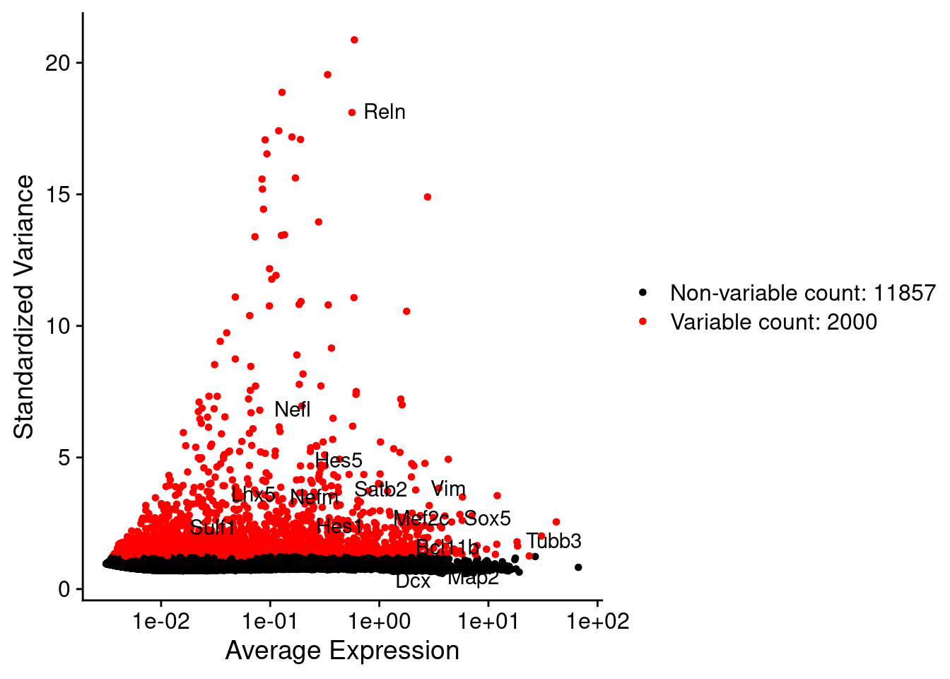
LabelPoints(plot = plot1, points = c(genesList$hk), repel = TRUE)
all.genes <- rownames(srat)
srat <- ScaleData(srat, features = all.genes)
seurat.data = GetAssayData(srat[["RNA"]],layer = "data")
corr.pval.list <- correlation_pvalues(data = seurat.data,
genesFromListExpressed,
n.cells = getNumCells(obj))
seurat.data.cor.big <- as.matrix(Matrix::forceSymmetric(corr.pval.list$data.cor, uplo = "U"))
htmp <- correlation_plot(seurat.data.cor.big,
genesList, title="Seurat corr")
p_values.fromSeurat <- corr.pval.list$p_values
seurat.data.cor.big <- corr.pval.list$data.cor
rm(corr.pval.list)
gc() used (Mb) gc trigger (Mb) max used (Mb)
Ncells 10178116 543.6 17741520 947.5 17741520 947.5
Vcells 354374909 2703.7 739832220 5644.5 763497772 5825.1draw(htmp, heatmap_legend_side="right")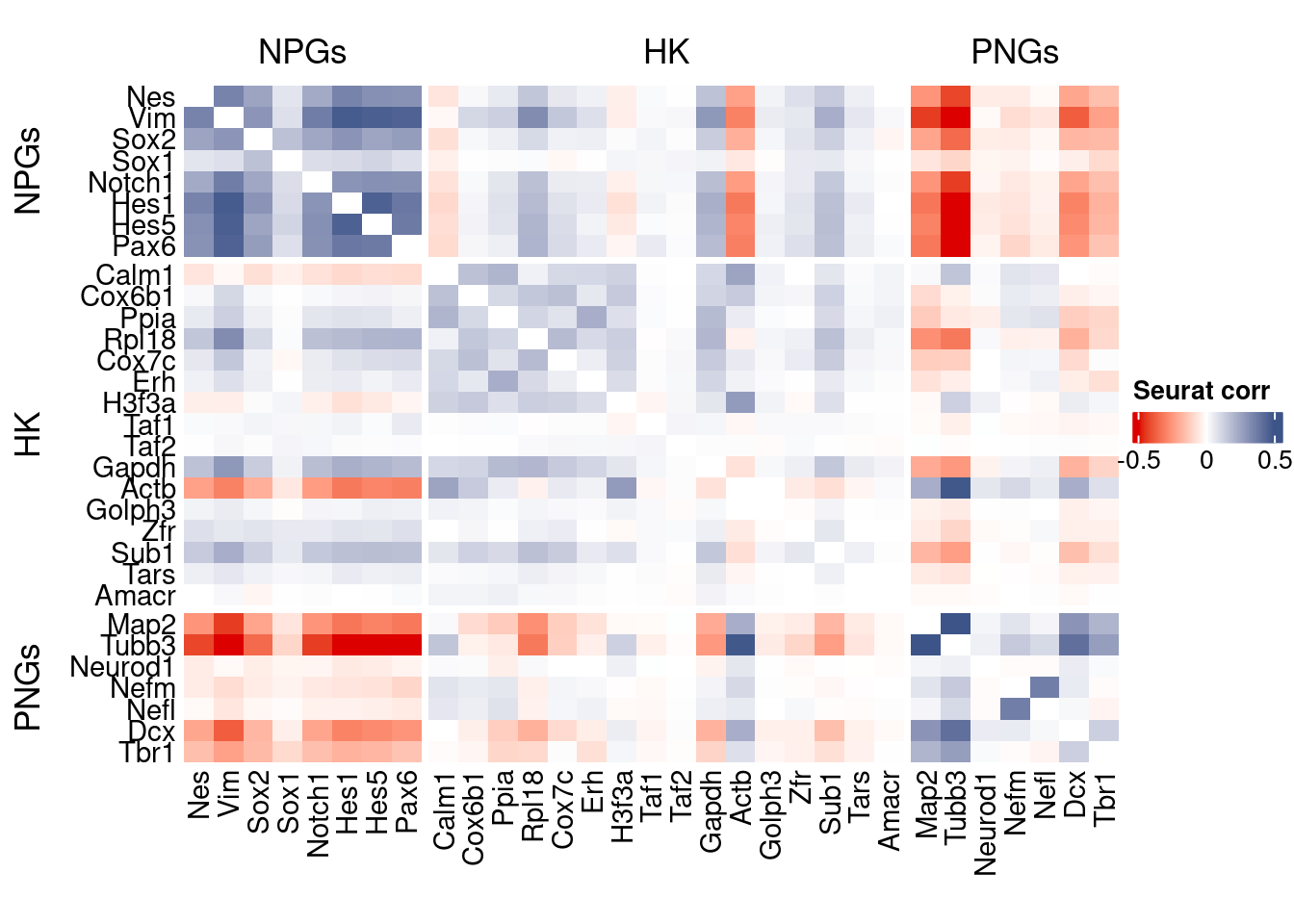
rm(seurat.data.cor.big)
rm(p_values.fromSeurat)
Seurat SC Transform
srat <-  SCTransform(srat,
                     method = "glmGamPoi",
                     vars.to.regress = "percent.mt",
                     verbose = FALSE)

seurat.data <- GetAssayData(srat[["SCT"]],layer = "data")

#Remove genes with all zeros
seurat.data <-seurat.data[rowSums(seurat.data) > 0,]


corr.pval.list <- correlation_pvalues(seurat.data,
                                      genesFromListExpressed,
                                      n.cells = getNumCells(obj))


seurat.data.cor.big <- as.matrix(Matrix::forceSymmetric(corr.pval.list$data.cor, uplo = "U"))

htmp <- correlation_plot(seurat.data.cor.big,
                         genesList, title="Seurat corr SCT")


p_values.fromSeurat <- corr.pval.list$p_values
seurat.data.cor.big <- corr.pval.list$data.cor

rm(corr.pval.list)
gc()
used (Mb) gc trigger (Mb) max used (Mb)
Ncells 10506648 561.2 17741520 947.5 17741520 947.5
Vcells 436644178 3331.4 1065534396 8129.4 1065526768 8129.4draw(htmp, heatmap_legend_side="right")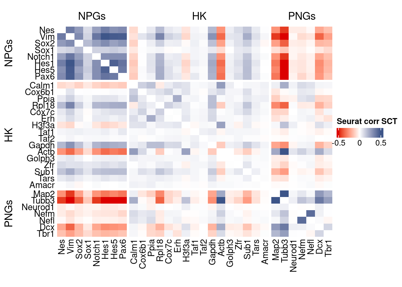
plot1 <- VariableFeaturePlot(srat)

plot1$data$centered_variance <- scale(plot1$data$residual_variance,
center = T,scale = F)write.csv(plot1$data,paste0("CoexData/",
"Variance_SeuratSCT_genes",
getMetadataElement(obj,
datasetTags()[["cond"]]),".csv"))
write_fst(as.data.frame(seurat.data.cor.big),path = paste0("CoexData/SeuratCorrSCT_",file_code,".fst"), compress = 100)
write_fst(as.data.frame(p_values.fromSeurat),path = paste0("CoexData/SeuratPValuesSCT_", file_code,".fst"))
write.csv(as.data.frame(p_values.fromSeurat),paste0("CoexData/SeuratPValuesSCT_", file_code,".csv"))
rm(seurat.data.cor.big)
rm(p_values.fromSeurat)Monocle
library(monocle3)cds <- new_cell_data_set(getRawData(obj),
cell_metadata = getMetadataCells(obj),
gene_metadata = getMetadataGenes(obj)
)
cds <- preprocess_cds(cds, num_dim = 100)
normalized_counts <- normalized_counts(cds)#Remove genes with all zeros
normalized_counts <- normalized_counts[rowSums(normalized_counts) > 0,]
corr.pval.list <- correlation_pvalues(normalized_counts,
genesFromListExpressed,
n.cells = getNumCells(obj))
rm(normalized_counts)
monocle.data.cor.big <- as.matrix(Matrix::forceSymmetric(corr.pval.list$data.cor, uplo = "U"))
htmp <- correlation_plot(data.cor.big = monocle.data.cor.big,
genesList,
title = "Monocle corr")
p_values.from.monocle <- corr.pval.list$p_values
monocle.data.cor.big <- corr.pval.list$data.cor
rm(corr.pval.list)
gc() used (Mb) gc trigger (Mb) max used (Mb)
Ncells 10692901 571.1 17741520 947.5 17741520 947.5
Vcells 439246749 3351.2 1065534396 8129.4 1065526768 8129.4draw(htmp, heatmap_legend_side="right")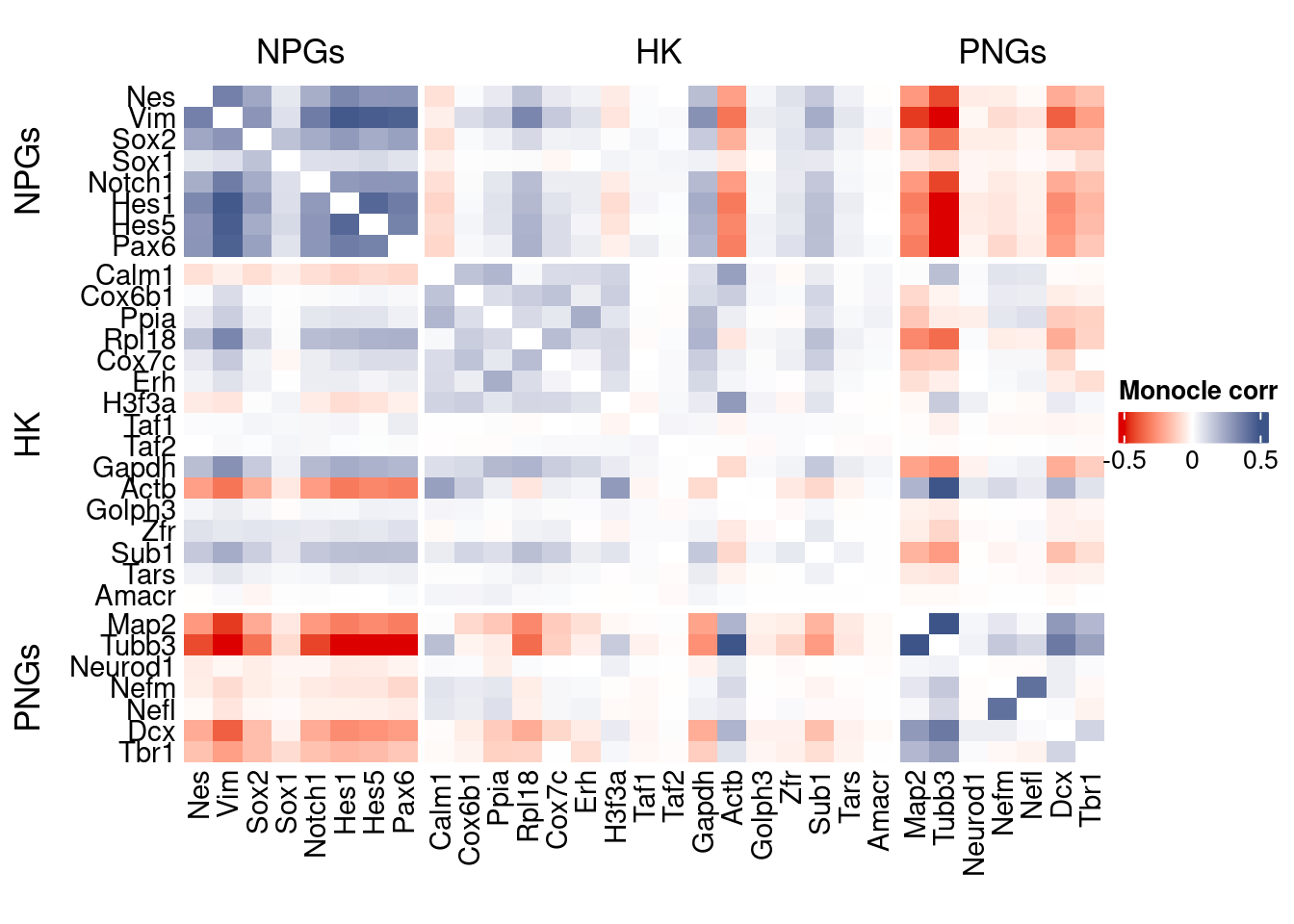
Cs-Core
library(CSCORE)Convert to Seurat obj
sceObj <- convertToSingleCellExperiment(obj)

# Correct: assay=NULL (or omit), data=NULL (since no logcounts)
seuratObj <- as.Seurat(
  x       = sceObj,
  counts  = "counts",
  data    = NULL,
  assay   = NULL,      # IMPORTANT: do NOT set to "RNA" here
  project = "COTAN"
)

# as.Seurat(SCE) creates assay "originalexp" by default; rename it to RNA
seuratObj <- RenameAssays(seuratObj, originalexp = "RNA", verbose = FALSE)
DefaultAssay(seuratObj) <- "RNA"

# Optional: keep COTAN payload
seuratObj@misc$COTAN <- S4Vectors::metadata(sceObj)
Extract CS_CORE corr matrix
#seuratObj@assays$RNA@counts <- ceiling(seuratObj@assays$RNA@counts)
csCoreRes <- CSCORE(seuratObj, genes = genesFromListExpressed)
[INFO] IRLS converged after 3 iterations.
[INFO] Starting WLS for covariance at Wed Jan 21 10:25:15 2026
[INFO] 0.0605% co-expression estimates were greater than 1 and were set to 1.
[INFO] 0.0000% co-expression estimates were smaller than -1 and were set to -1.
[INFO] Finished WLS. Elapsed time: 0.2305 seconds.mat <- as.matrix(csCoreRes$est)
diag(mat) <- 0
split.genes <- base::factor(c(rep("NPGs",sum(genesList[["NPGs"]] %in% genesFromListExpressed)),
rep("HK",sum(genesList[["hk"]] %in% genesFromListExpressed)),
rep("PNGs",sum(genesList[["PNGs"]] %in% genesFromListExpressed))
),
levels = c("NPGs","HK","PNGs"))
f1 = colorRamp2(seq(-0.5,0.5, length = 3), c("#DC0000B2", "white","#3C5488B2" ))
htmp <- Heatmap(as.matrix(mat[c(genesList$NPGs,genesList$hk,genesList$PNGs),c(genesList$NPGs,genesList$hk,genesList$PNGs)]),
#width = ncol(coexMat)*unit(2.5, "mm"),
height = nrow(mat)*unit(3, "mm"),
cluster_rows = FALSE,
cluster_columns = FALSE,
col = f1,
row_names_side = "left",
row_names_gp = gpar(fontsize = 11),
column_names_gp = gpar(fontsize = 11),
column_split = split.genes,
row_split = split.genes,
cluster_row_slices = FALSE,
cluster_column_slices = FALSE,
heatmap_legend_param = list(
title = "CS-CORE", at = c(-0.5, 0, 0.5),
direction = "horizontal",
labels = c("-0.5", "0", "0.5")
)
)
draw(htmp, heatmap_legend_side="right")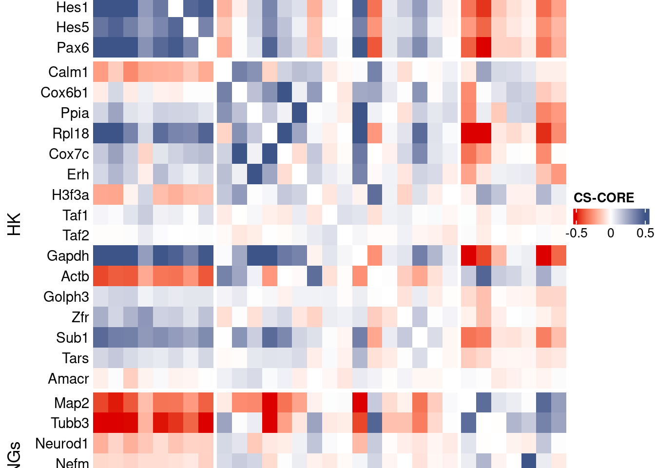
Save CS_CORE matrix
write_fst(as.data.frame(csCoreRes$est), path = paste0("CoexData/CS_CORECorr_", file_code,".fst"),compress = 100)
write_fst(as.data.frame(csCoreRes$p_value), path = paste0("CoexData/CS_COREPValues_", file_code,".fst"),compress = 100)
write.csv(as.data.frame(csCoreRes$p_value), paste0("CoexData/CS_COREPValues_", file_code,".csv"))
Baseline: Spearman on UMI counts
corr.pval.list <- correlation_pvaluesSpearman(data = getRawData(obj),
                                      genesFromListExpressed,
                                      n.cells = getNumCells(obj))

data.cor.big <- as.matrix(Matrix::forceSymmetric(corr.pval.list$data.cor, uplo = "U"))

htmp <- correlation_plot(data.cor.big,
                         genesList, title="UMI baseline S. corr")


p_values.fromSp.C <- corr.pval.list$p_values
data.cor.bigSp.C <- corr.pval.list$data.cor

rm(corr.pval.list)
gc()
used (Mb) gc trigger (Mb) max used (Mb)
Ncells 10701612 571.6 17741520 947.5 17741520 947.5
Vcells 439748623 3355.1 1065534396 8129.4 1065526768 8129.4draw(htmp, heatmap_legend_side="right")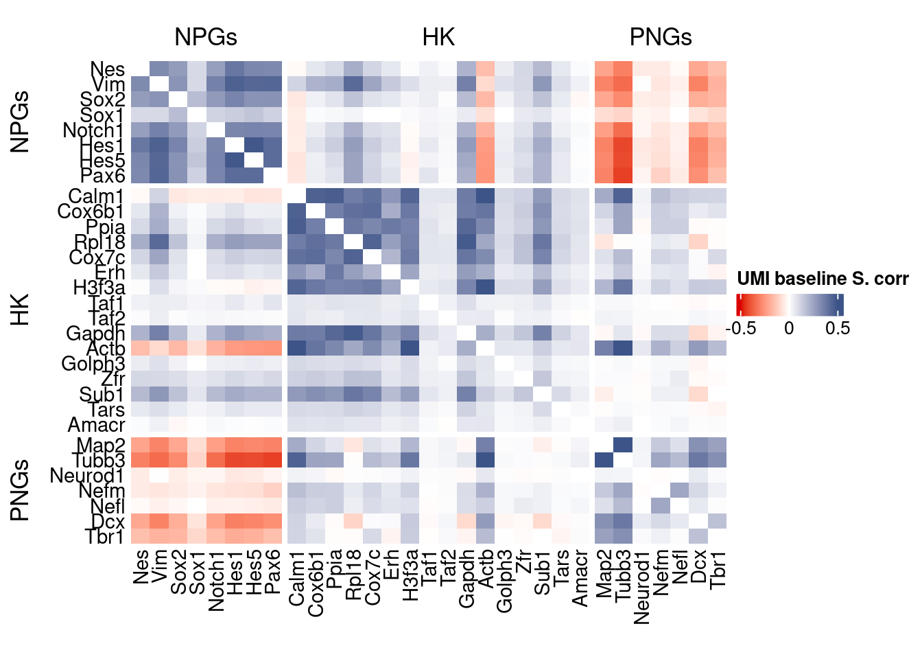
write.csv(as.data.frame(p_values.fromSp.C), paste0("CoexData/BaselineUMISpCorrPValues_", file_code,".csv"))Baseline: Pearson on binarized counts
corr.pval.list <- correlation_pvalues(data = getZeroOneProj(obj),
                                      genesFromListExpressed,
                                      n.cells = getNumCells(obj))

data.cor.big <- as.matrix(Matrix::forceSymmetric(corr.pval.list$data.cor, uplo = "U"))

htmp <- correlation_plot(data.cor.big,
                         genesList, title="Zero-one P. corr")


p_values.fromSp.C <- corr.pval.list$p_values
data.cor.bigSp.C <- corr.pval.list$data.cor

rm(corr.pval.list)
gc()
used (Mb) gc trigger (Mb) max used (Mb)
Ncells 10701739 571.6 17741520 947.5 17741520 947.5
Vcells 439748881 3355.1 1065534396 8129.4 1065526768 8129.4draw(htmp, heatmap_legend_side="right")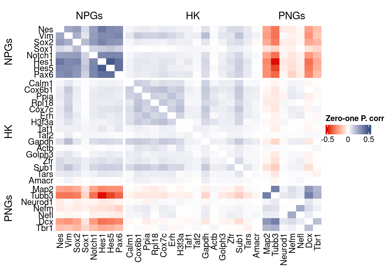
write.csv(as.data.frame(p_values.fromSp.C), paste0("CoexData/ZeroOnePCorrPValues_", file_code,".csv"))Sys.time()[1] "2026-01-21 10:25:25 CET"sessionInfo()R version 4.5.2 (2025-10-31)
Platform: x86_64-pc-linux-gnu
Running under: Ubuntu 22.04.5 LTS
Matrix products: default
BLAS: /usr/lib/x86_64-linux-gnu/blas/libblas.so.3.10.0
LAPACK: /usr/lib/x86_64-linux-gnu/lapack/liblapack.so.3.10.0 LAPACK version 3.10.0
locale:
[1] LC_CTYPE=C.UTF-8 LC_NUMERIC=C LC_TIME=C.UTF-8
[4] LC_COLLATE=C.UTF-8 LC_MONETARY=C.UTF-8 LC_MESSAGES=C.UTF-8
[7] LC_PAPER=C.UTF-8 LC_NAME=C LC_ADDRESS=C
[10] LC_TELEPHONE=C LC_MEASUREMENT=C.UTF-8 LC_IDENTIFICATION=C
time zone: Europe/Rome
tzcode source: system (glibc)
attached base packages:
[1] stats4 parallel grid stats graphics grDevices utils
[8] datasets methods base
other attached packages:
[1] CSCORE_1.0.2 monocle3_1.3.7
[3] SingleCellExperiment_1.32.0 SummarizedExperiment_1.38.1
[5] GenomicRanges_1.62.1 Seqinfo_1.0.0
[7] IRanges_2.44.0 S4Vectors_0.48.0
[9] MatrixGenerics_1.22.0 matrixStats_1.5.0
[11] Biobase_2.70.0 BiocGenerics_0.56.0
[13] generics_0.1.3 fstcore_0.10.0
[15] fst_0.9.8 stringr_1.6.0
[17] HiClimR_2.2.1 doParallel_1.0.17
[19] iterators_1.0.14 foreach_1.5.2
[21] Rfast_2.1.5.1 RcppParallel_5.1.10
[23] zigg_0.0.2 Rcpp_1.1.0
[25] patchwork_1.3.2 Seurat_5.4.0
[27] SeuratObject_5.3.0 sp_2.2-0
[29] Hmisc_5.2-3 dplyr_1.1.4
[31] circlize_0.4.16 ComplexHeatmap_2.26.0
[33] COTAN_2.11.1
loaded via a namespace (and not attached):
[1] RcppAnnoy_0.0.22 splines_4.5.2
[3] later_1.4.2 tibble_3.3.0
[5] polyclip_1.10-7 rpart_4.1.24
[7] fastDummies_1.7.5 lifecycle_1.0.4
[9] Rdpack_2.6.4 globals_0.18.0
[11] lattice_0.22-7 MASS_7.3-65
[13] backports_1.5.0 ggdist_3.3.3
[15] dendextend_1.19.0 magrittr_2.0.4
[17] plotly_4.11.0 rmarkdown_2.29
[19] yaml_2.3.10 httpuv_1.6.16
[21] otel_0.2.0 glmGamPoi_1.20.0
[23] sctransform_0.4.2 spam_2.11-1
[25] spatstat.sparse_3.1-0 reticulate_1.44.1
[27] minqa_1.2.8 cowplot_1.2.0
[29] pbapply_1.7-2 RColorBrewer_1.1-3
[31] abind_1.4-8 Rtsne_0.17
[33] purrr_1.2.0 nnet_7.3-20
[35] GenomeInfoDbData_1.2.14 ggrepel_0.9.6
[37] irlba_2.3.5.1 listenv_0.10.0
[39] spatstat.utils_3.2-1 goftest_1.2-3
[41] RSpectra_0.16-2 spatstat.random_3.4-3
[43] fitdistrplus_1.2-2 parallelly_1.46.0
[45] DelayedMatrixStats_1.30.0 ncdf4_1.24
[47] codetools_0.2-20 DelayedArray_0.36.0
[49] tidyselect_1.2.1 shape_1.4.6.1
[51] UCSC.utils_1.4.0 farver_2.1.2
[53] lme4_1.1-37 ScaledMatrix_1.16.0
[55] viridis_0.6.5 base64enc_0.1-3
[57] spatstat.explore_3.6-0 jsonlite_2.0.0
[59] GetoptLong_1.1.0 Formula_1.2-5
[61] progressr_0.18.0 ggridges_0.5.6
[63] survival_3.8-3 tools_4.5.2
[65] ica_1.0-3 glue_1.8.0
[67] gridExtra_2.3 SparseArray_1.10.8
[69] xfun_0.52 distributional_0.6.0
[71] ggthemes_5.2.0 GenomeInfoDb_1.44.0
[73] withr_3.0.2 fastmap_1.2.0
[75] boot_1.3-32 digest_0.6.37
[77] rsvd_1.0.5 parallelDist_0.2.6
[79] R6_2.6.1 mime_0.13
[81] colorspace_2.1-1 Cairo_1.7-0
[83] scattermore_1.2 tensor_1.5
[85] spatstat.data_3.1-9 tidyr_1.3.1
[87] data.table_1.18.0 httr_1.4.7
[89] htmlwidgets_1.6.4 S4Arrays_1.10.1
[91] uwot_0.2.3 pkgconfig_2.0.3
[93] gtable_0.3.6 lmtest_0.9-40
[95] S7_0.2.1 XVector_0.50.0
[97] htmltools_0.5.8.1 dotCall64_1.2
[99] clue_0.3-66 scales_1.4.0
[101] png_0.1-8 reformulas_0.4.1
[103] spatstat.univar_3.1-6 rstudioapi_0.18.0
[105] knitr_1.50 reshape2_1.4.4
[107] rjson_0.2.23 nloptr_2.2.1
[109] checkmate_2.3.2 nlme_3.1-168
[111] proxy_0.4-29 zoo_1.8-14
[113] GlobalOptions_0.1.2 KernSmooth_2.23-26
[115] miniUI_0.1.2 foreign_0.8-90
[117] pillar_1.11.1 vctrs_0.7.0
[119] RANN_2.6.2 promises_1.5.0
[121] BiocSingular_1.26.1 beachmat_2.26.0
[123] xtable_1.8-4 cluster_2.1.8.1
[125] htmlTable_2.4.3 evaluate_1.0.5
[127] magick_2.9.0 zeallot_0.2.0
[129] cli_3.6.5 compiler_4.5.2
[131] rlang_1.1.7 crayon_1.5.3
[133] future.apply_1.20.0 labeling_0.4.3
[135] plyr_1.8.9 stringi_1.8.7
[137] viridisLite_0.4.2 deldir_2.0-4
[139] BiocParallel_1.44.0 assertthat_0.2.1
[141] lazyeval_0.2.2 spatstat.geom_3.6-1
[143] Matrix_1.7-4 RcppHNSW_0.6.0
[145] sparseMatrixStats_1.20.0 future_1.69.0
[147] ggplot2_4.0.1 shiny_1.12.1
[149] rbibutils_2.3 ROCR_1.0-11
[151] igraph_2.2.1