options(parallelly.fork.enable = TRUE)
library(COTAN)
library(zeallot)
library(data.table)
library(factoextra)
library(Rtsne)
library(qpdf)
library(stringr)E14.5 Mouse Cortex Loo 2019
e14_dge = read.table("Data/MouseCortex/OriginalData/E14_combined_matrix.txt.gz",header=T,sep="\t",row.names=1)

print(dim(e14_dge))
[1] 21313 11069outDir <- "Data/MouseCortex/"
setLoggingLevel(1)
setLoggingFile(file.path(outDir, "Dataset.log"))cond <- "MouseCortex_E14.5"
obj <- COTAN(raw = e14_dge)
obj <- initializeMetaDataset(obj,
GEO = "GSE123335",
sequencingMethod = "Drop_seq",
sampleCondition = cond)
CellCond <- str_split(getCells(obj),pattern = "_",simplify = T)[,1]
names(CellCond) <- getCells(obj)
obj <- addCondition(obj,"CellCond",CellCond)
rm(e14_dge)ECDPlot(obj, yCut = 400L)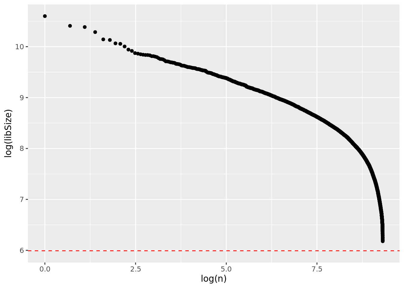
cellSizePlot(obj,condName = "CellCond")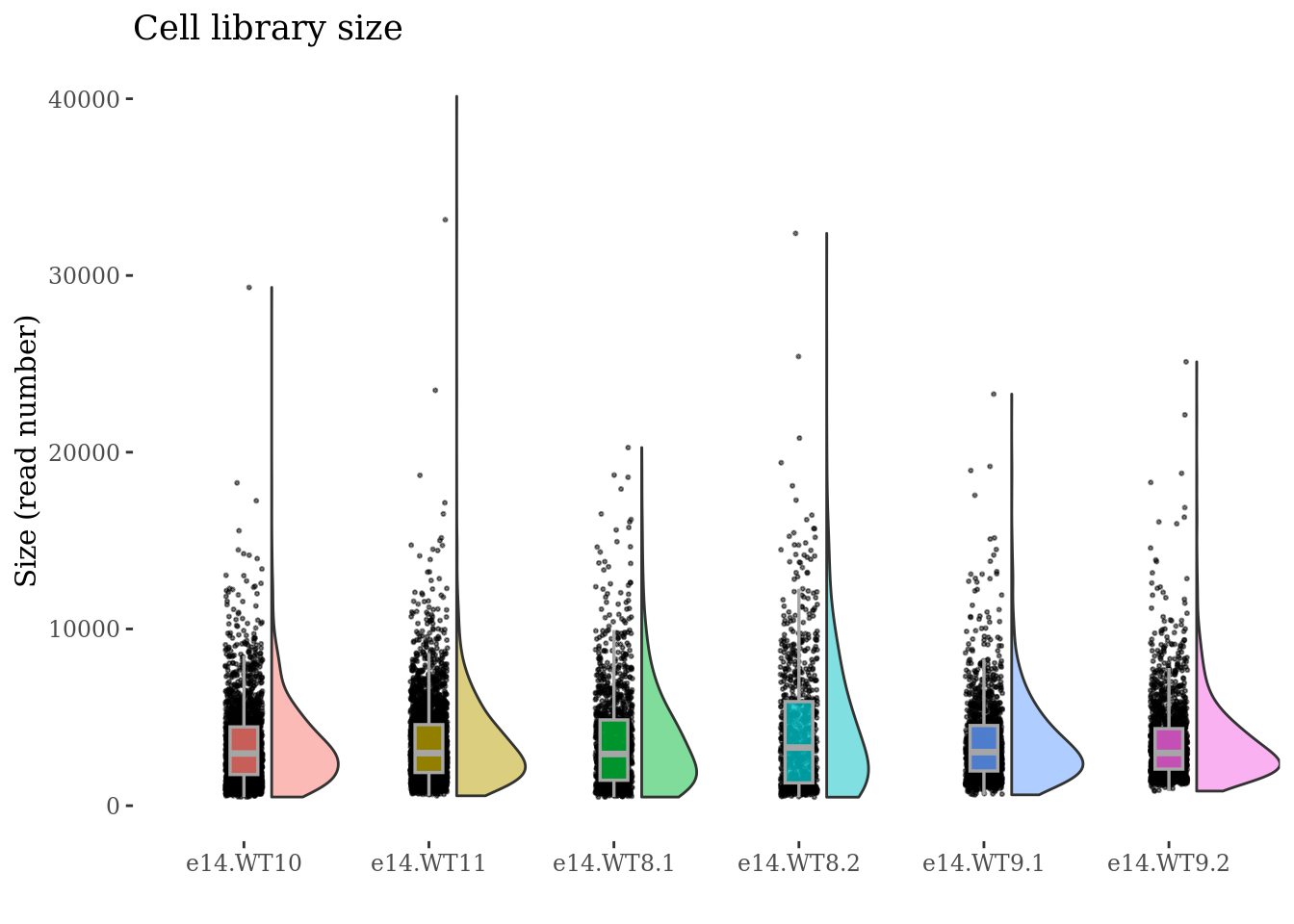
genesSizePlot(obj,condName = "CellCond")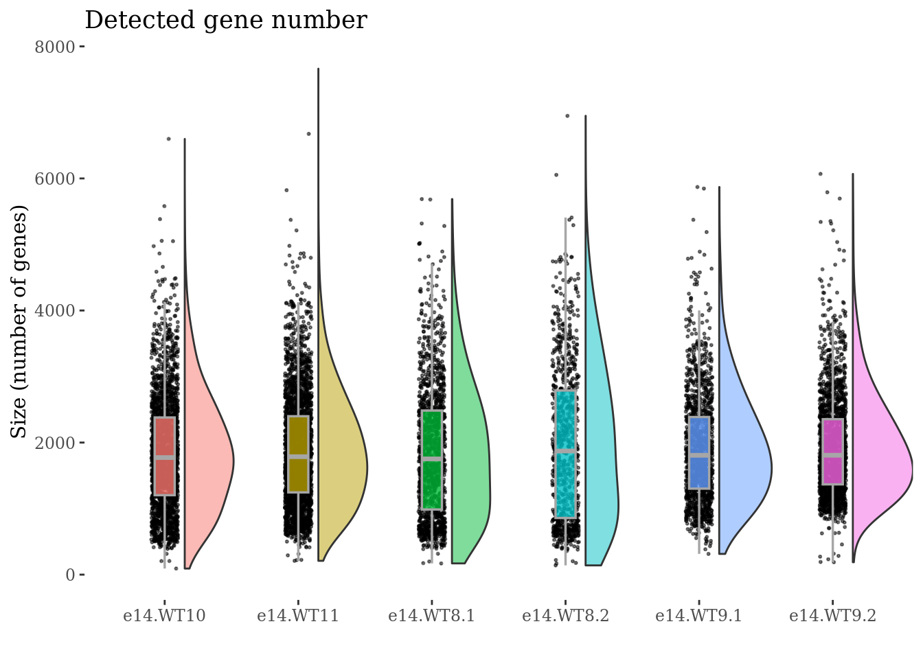
mit <- mitochondrialPercentagePlot(obj, genePrefix = "^mt-",condName = "CellCond")
mit[["plot"]]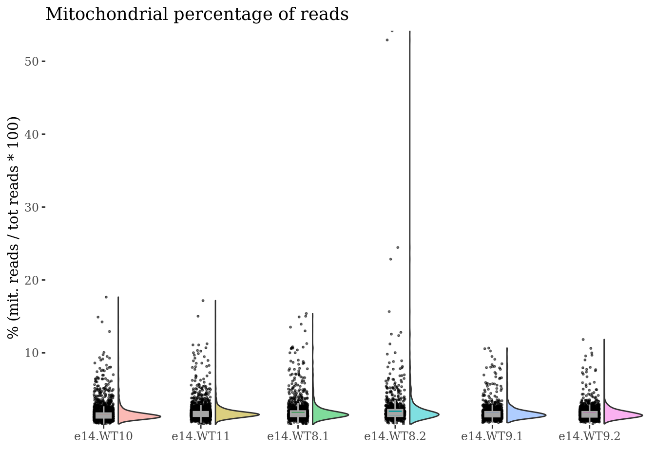
To drop cells by cell library size:
cells_to_rem <- getCells(obj)[getCellsSize(obj) > 15000]
obj <- dropGenesCells(obj, cells = cells_to_rem)
cellSizePlot(obj,condName = "CellCond")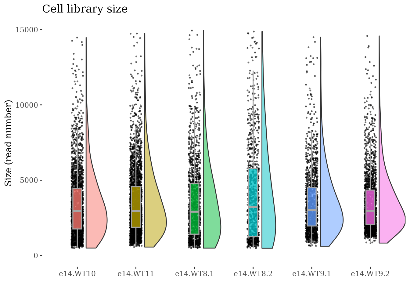
genesSizePlot(obj,condName = "CellCond")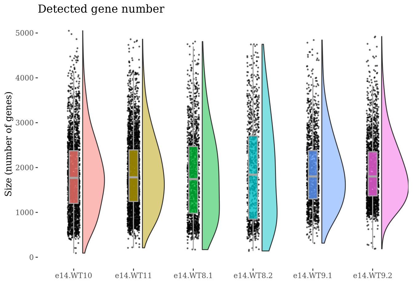
To drop cells by mitochondrial percentage:
to_rem <- mit[["sizes"]][["mit.percentage"]] > 7.5
cells_to_rem <- rownames(mit[["sizes"]])[to_rem]
obj <- dropGenesCells(obj, cells = cells_to_rem)

mit <- mitochondrialPercentagePlot(obj, genePrefix = "^mt-",condName = "CellCond")

mit[["plot"]]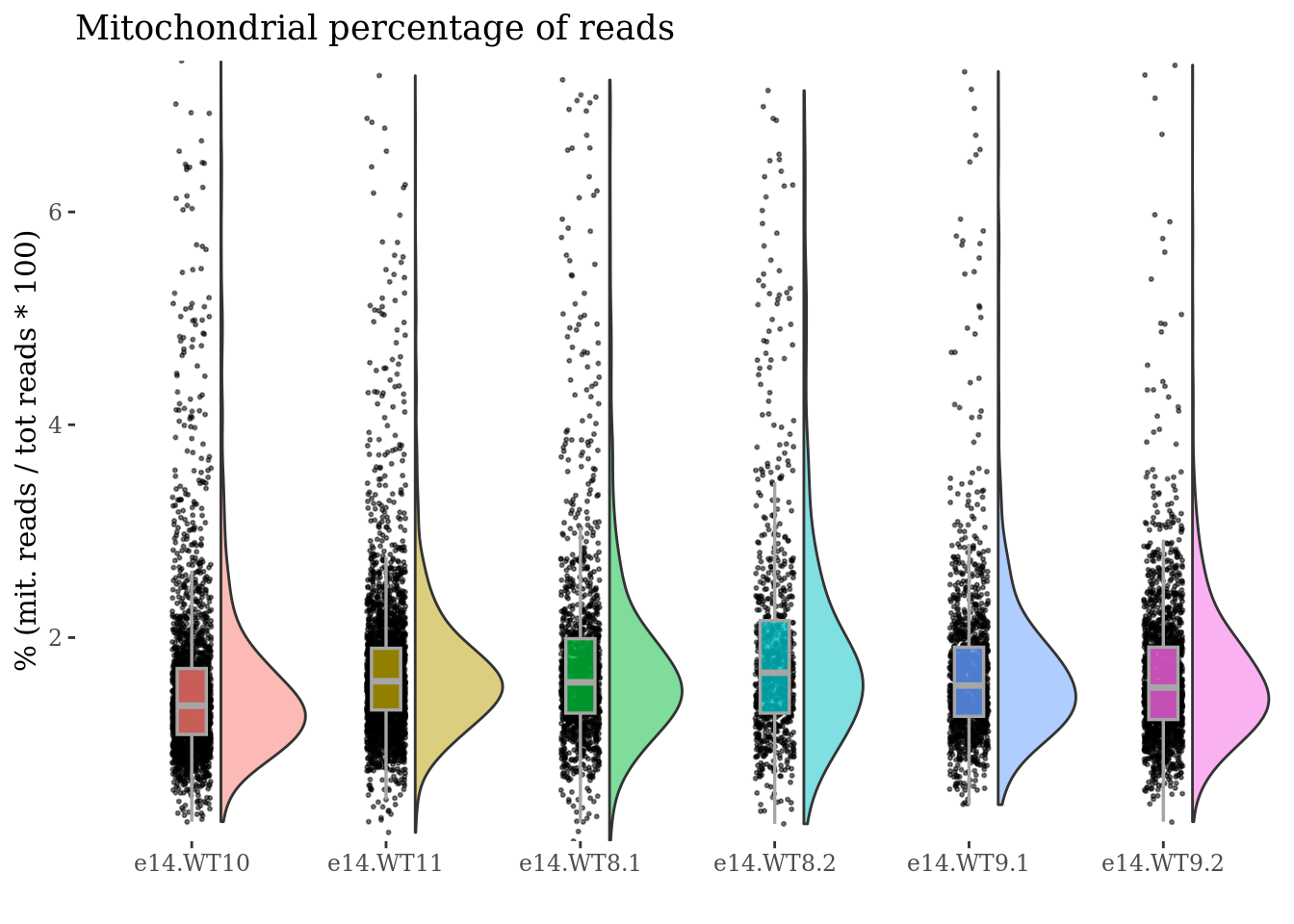
cellSizePlot(obj,condName = "CellCond")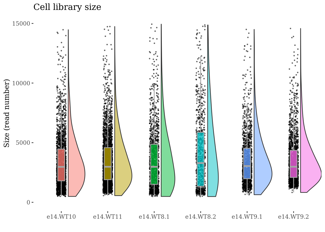
obj <- clean(obj)
c(pcaCellsPlot, pcaCellsData, genesPlot, UDEPlot, nuPlot, zoom) %<-% cleanPlots(obj)

pcaCellsPlot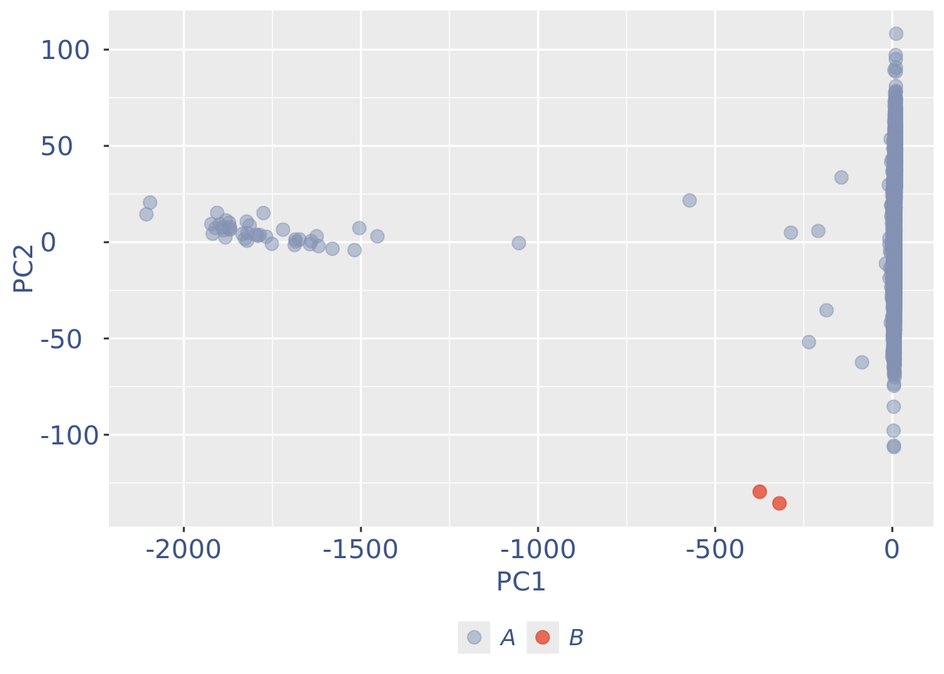
genesPlot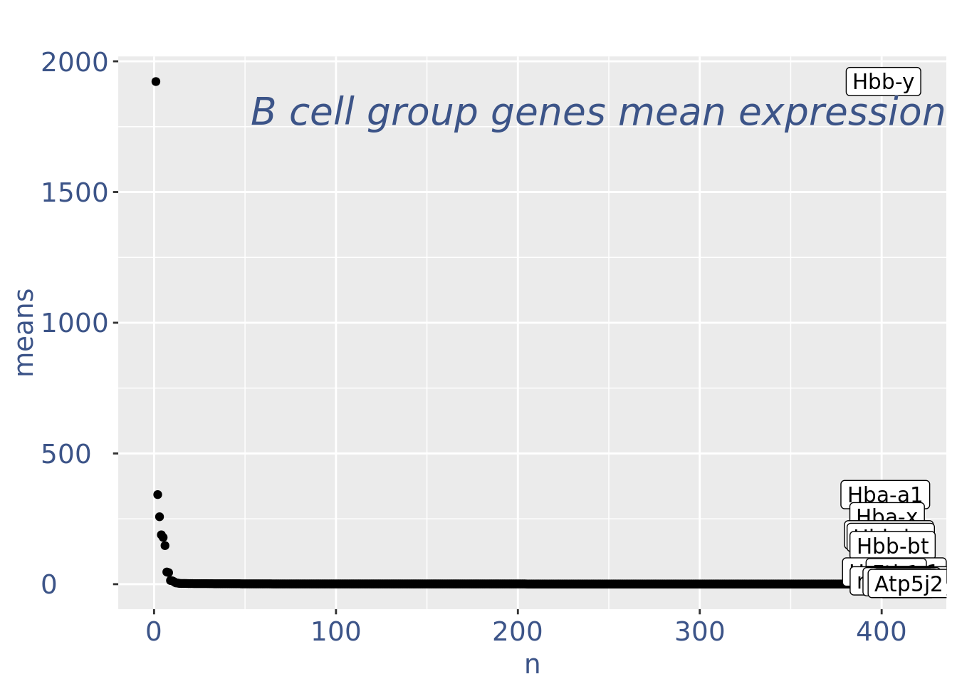
cells_to_rem <- rownames(pcaCellsData)[pcaCellsData[["groups"]] == "B"]
obj <- dropGenesCells(obj, cells = cells_to_rem)
obj <- clean(obj)
c(pcaCellsPlot, pcaCellsData, genesPlot, UDEPlot, nuPlot, zoom) %<-% cleanPlots(obj)

pcaCellsPlot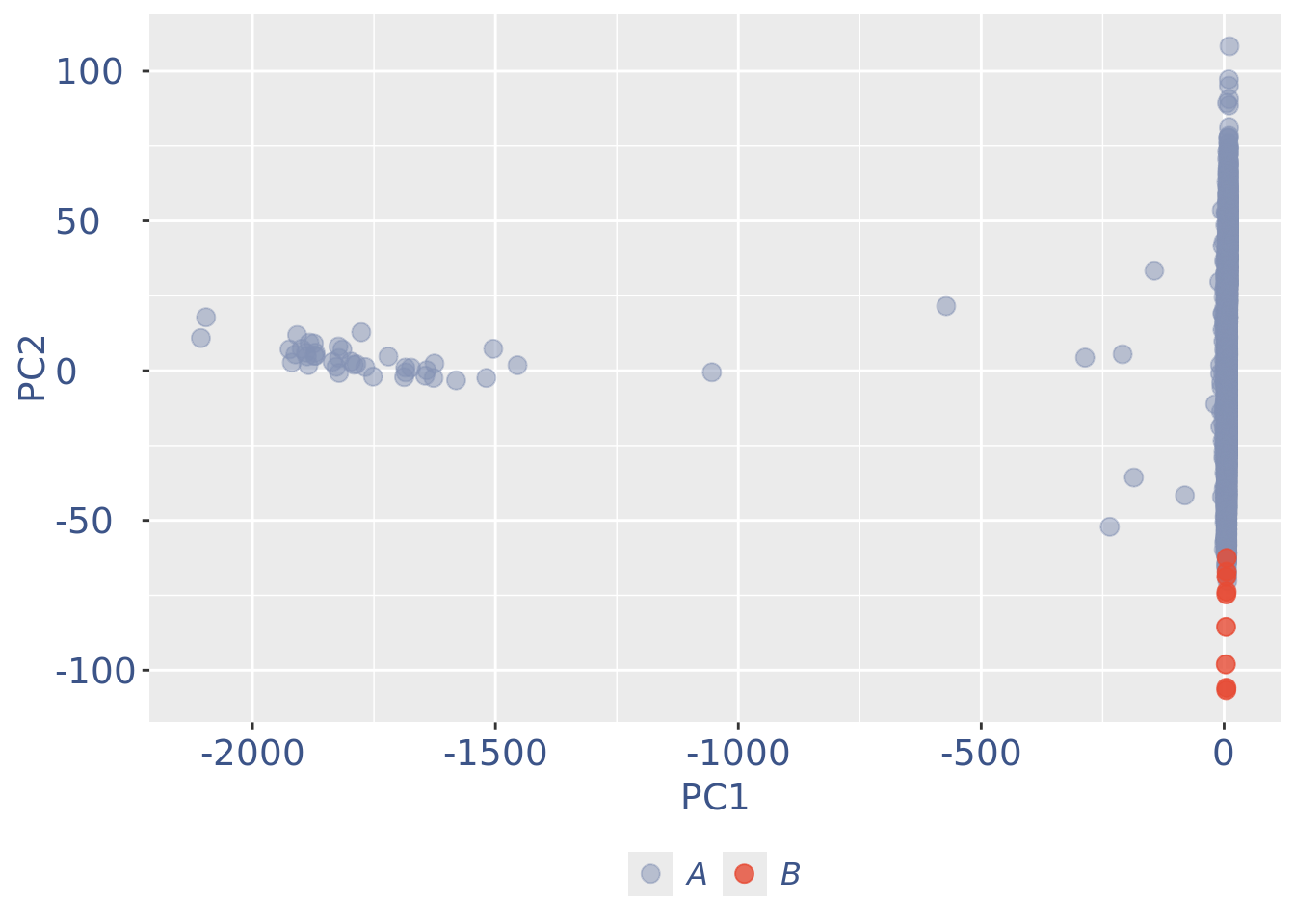
genesPlot
plot(nuPlot)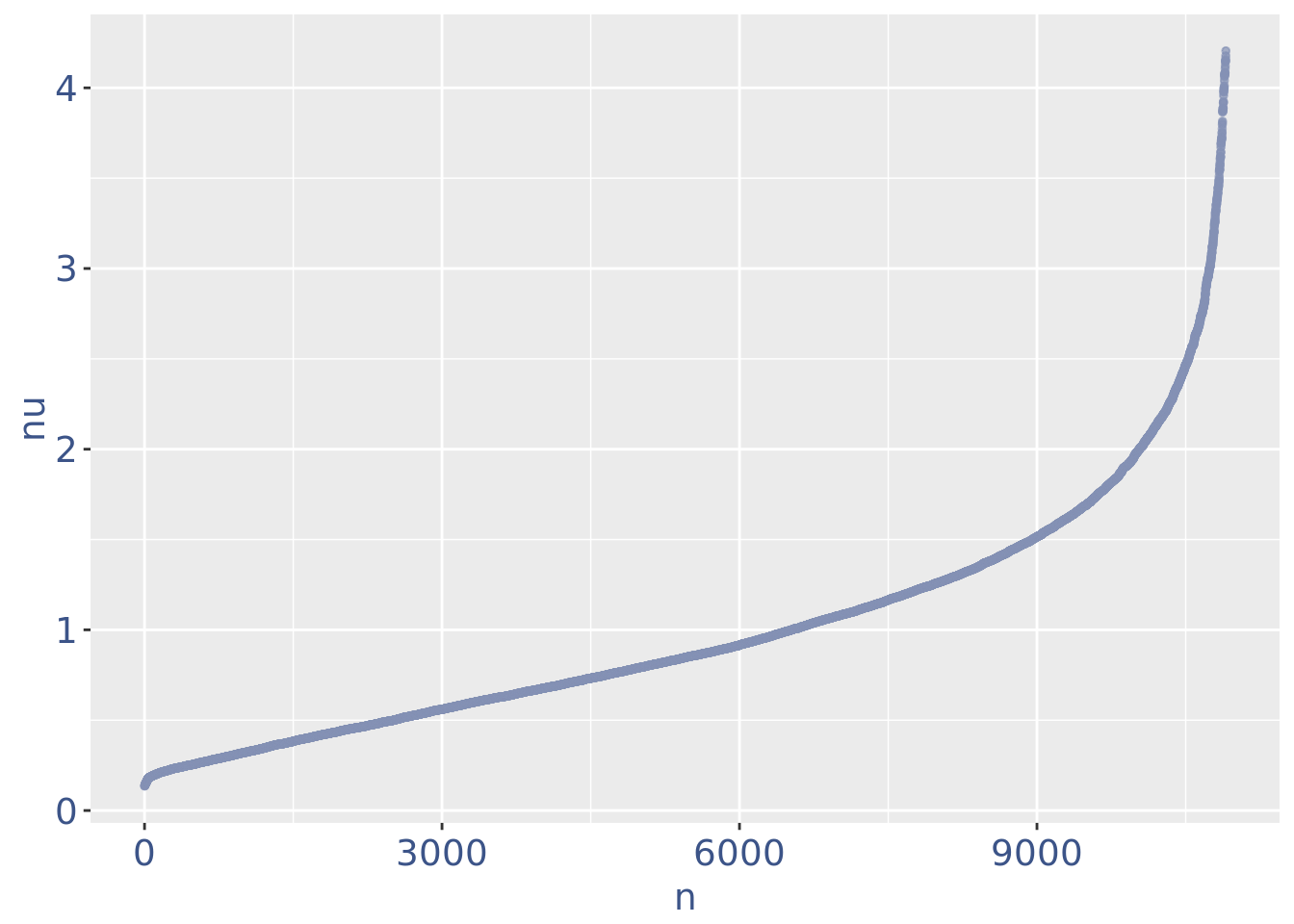
nuDf <- data.frame("nu" = sort(getNu(obj)), "n" = seq_along(getNu(obj)))
yset <- 0.18 # the threshold to remove low UDE cells
plot.ude <- ggplot(nuDf, aes(x = n, y = nu)) +
            geom_point(colour = "#8491B4B2", size = 1.0) +
            xlim(0L, 3000) +
            ylim(0.0, 1.0) +
            geom_hline(yintercept = yset, linetype = "dashed",
                       color = "darkred") +
            annotate(geom = "text", x = 1000L, y = 0.25,
                     label = paste0("to remove cells with nu < ", yset),
                     color = "darkred", size = 4.5)

plot.ude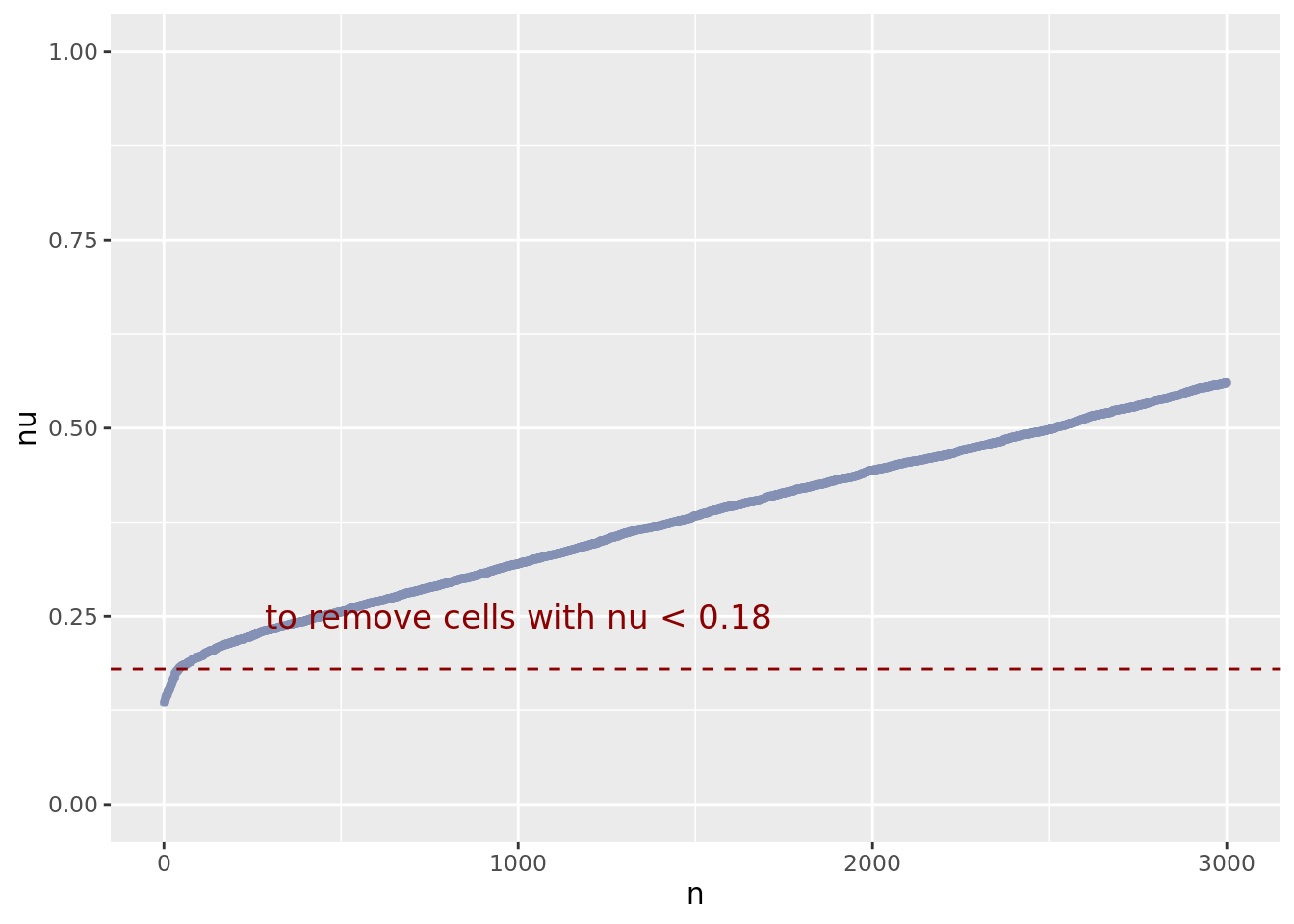
obj <- addElementToMetaDataset(obj, "Threshold low UDE cells:", yset)

cells_to_rem <- rownames(nuDf)[nuDf[["nu"]] < yset]
obj <- dropGenesCells(obj, cells = cells_to_rem)
obj <- clean(obj)
c(pcaCellsPlot, pcaCellsData, genesPlot, UDEPlot, nuPlot, zoom) %<-% cleanPlots(obj)

pcaCellsPlot
genesPlot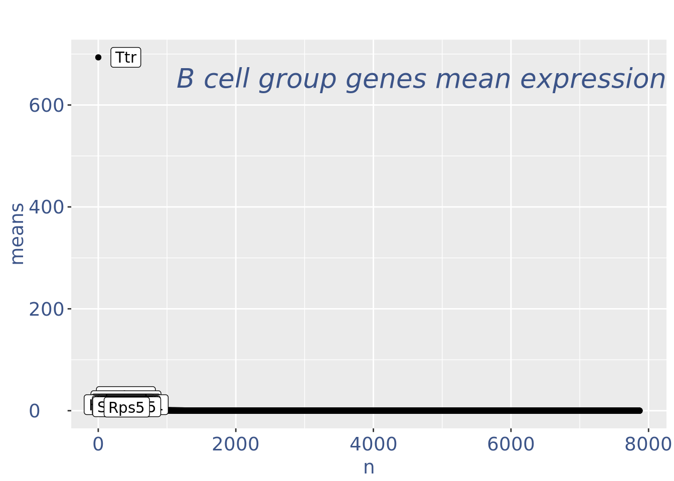
UDEPlot
nuPlot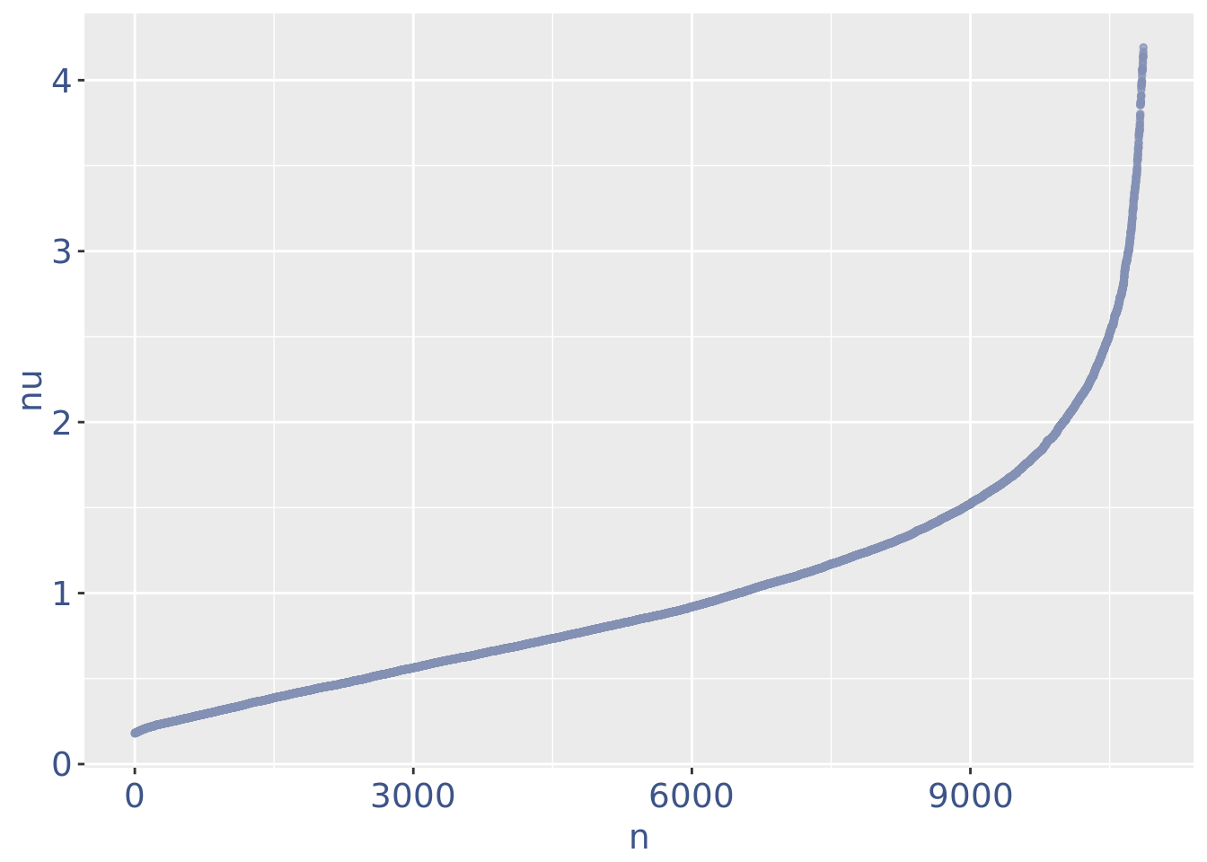
UDEPlot$data$Sample <- str_split(rownames(UDEPlot$data),pattern = "_",simplify = T)[,1]

ggplot(UDEPlot$data, aes(PC1,PC2,color = Sample)) + geom_point(size = 0.5, alpha=0.7)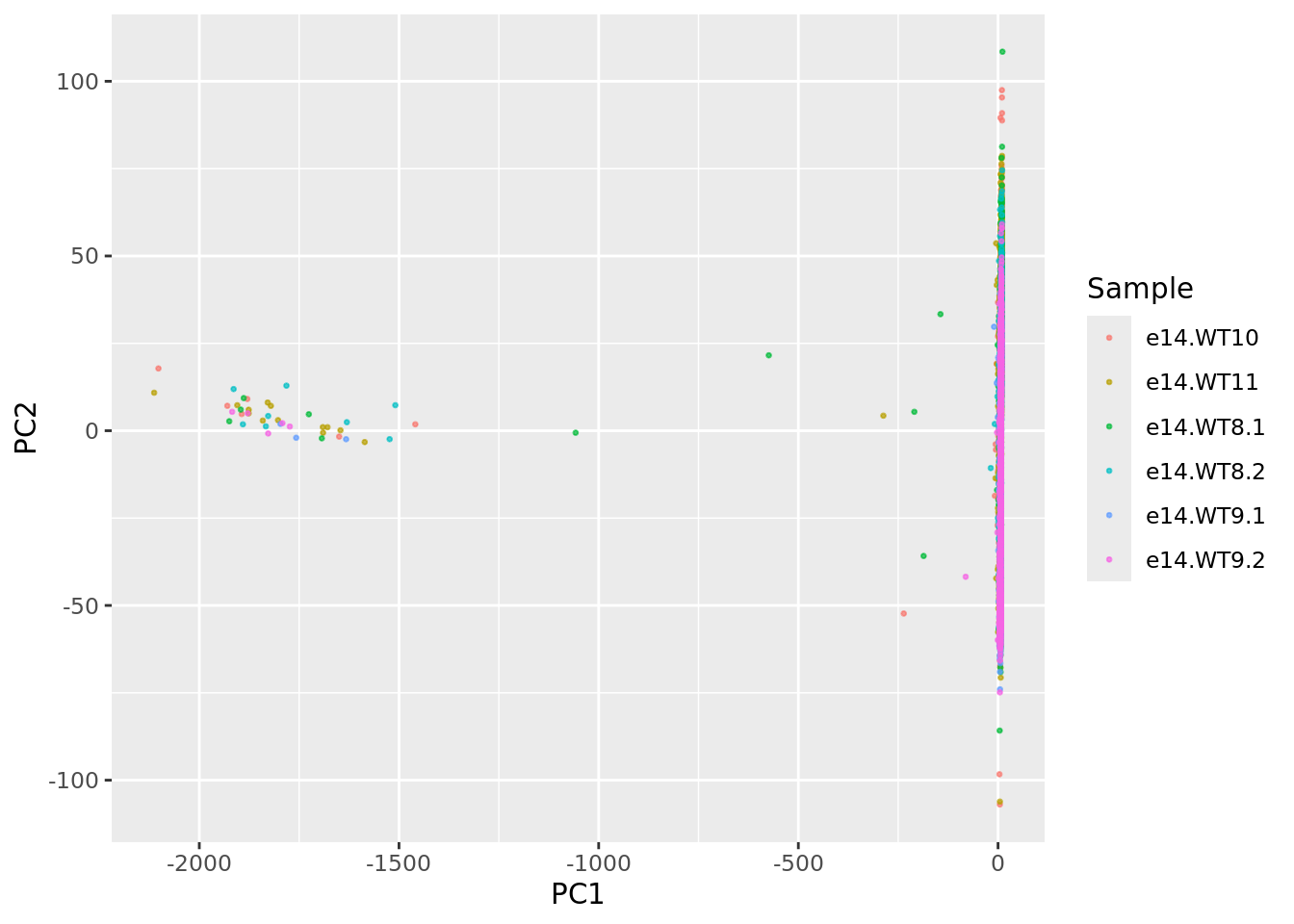
ggplot(UDEPlot$data, aes(PC2,PC3,color = Sample)) + geom_point(size = 0.5, alpha=0.7)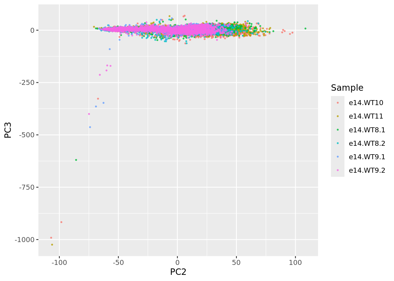
ggplot(UDEPlot$data, aes(PC2,PC5,color = Sample)) + geom_point(size = 0.5, alpha=0.7)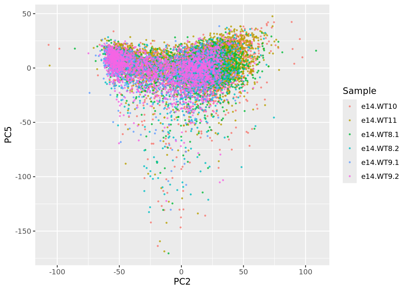
ggplot(UDEPlot$data, aes(PC2,PC5,color = groups)) + geom_point(size = 0.5, alpha=0.7)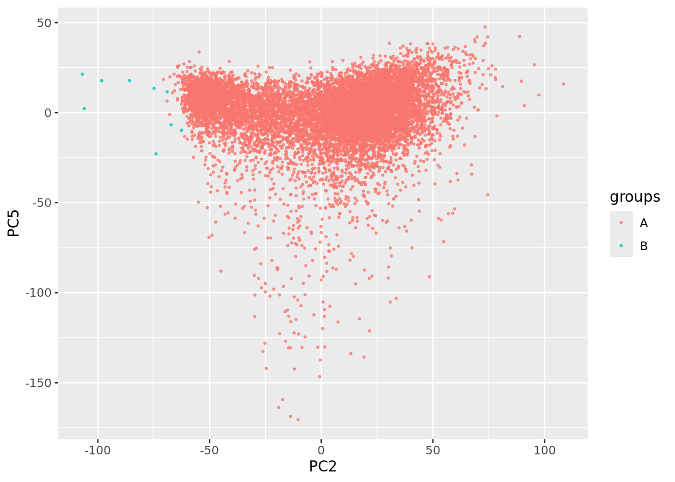
COTAN analysis
In this part, all the contingency tables are computed and used to get the statistics.
obj <- estimateLambdaLinear(obj)
obj <- estimateDispersionBisection(obj, cores = 15L)
COEX evaluation and storing
obj <- calculateCoex(obj)# saving the structure
saveRDS(obj, file = file.path(outDir, paste0(cond, ".cotan.RDS")))objTemp <- obj
obj <- readRDS(file = file.path(outDir, paste0(cond, ".cotan.RDS")))(Next code… just check that the already stored data is identical to the re-calculated)
identical(getRawData(obj),getRawData(objTemp))[1] TRUEsessionInfo()R version 4.5.2 (2025-10-31)
Platform: x86_64-pc-linux-gnu
Running under: Ubuntu 22.04.5 LTS
Matrix products: default
BLAS: /usr/lib/x86_64-linux-gnu/blas/libblas.so.3.10.0
LAPACK: /usr/lib/x86_64-linux-gnu/lapack/liblapack.so.3.10.0 LAPACK version 3.10.0
locale:
[1] LC_CTYPE=C.UTF-8 LC_NUMERIC=C LC_TIME=C.UTF-8
[4] LC_COLLATE=C.UTF-8 LC_MONETARY=C.UTF-8 LC_MESSAGES=C.UTF-8
[7] LC_PAPER=C.UTF-8 LC_NAME=C LC_ADDRESS=C
[10] LC_TELEPHONE=C LC_MEASUREMENT=C.UTF-8 LC_IDENTIFICATION=C
time zone: Europe/Rome
tzcode source: system (glibc)
attached base packages:
[1] stats graphics grDevices utils datasets methods base
other attached packages:
[1] stringr_1.5.1 qpdf_1.3.5 Rtsne_0.17 factoextra_1.0.7
[5] ggplot2_4.0.1 data.table_1.17.0 zeallot_0.2.0 COTAN_2.9.4
loaded via a namespace (and not attached):
[1] RcppAnnoy_0.0.22 splines_4.5.2
[3] later_1.4.2 tibble_3.3.0
[5] polyclip_1.10-7 fastDummies_1.7.5
[7] lifecycle_1.0.4 doParallel_1.0.17
[9] globals_0.18.0 lattice_0.22-7
[11] MASS_7.3-65 dendextend_1.19.0
[13] magrittr_2.0.4 plotly_4.11.0
[15] rmarkdown_2.29 yaml_2.3.10
[17] httpuv_1.6.16 Seurat_5.2.1
[19] sctransform_0.4.2 askpass_1.2.1
[21] spam_2.11-1 sp_2.2-0
[23] spatstat.sparse_3.1-0 reticulate_1.42.0
[25] cowplot_1.1.3 pbapply_1.7-2
[27] RColorBrewer_1.1-3 abind_1.4-8
[29] GenomicRanges_1.60.0 purrr_1.2.0
[31] BiocGenerics_0.54.0 circlize_0.4.16
[33] GenomeInfoDbData_1.2.14 IRanges_2.42.0
[35] S4Vectors_0.46.0 ggrepel_0.9.6
[37] irlba_2.3.5.1 listenv_0.9.1
[39] spatstat.utils_3.1-4 goftest_1.2-3
[41] RSpectra_0.16-2 spatstat.random_3.4-1
[43] fitdistrplus_1.2-2 parallelly_1.45.0
[45] codetools_0.2-20 DelayedArray_0.34.1
[47] tidyselect_1.2.1 shape_1.4.6.1
[49] UCSC.utils_1.4.0 farver_2.1.2
[51] ScaledMatrix_1.16.0 viridis_0.6.5
[53] matrixStats_1.5.0 stats4_4.5.2
[55] spatstat.explore_3.4-2 jsonlite_2.0.0
[57] GetoptLong_1.0.5 gghalves_0.1.4
[59] progressr_0.15.1 ggridges_0.5.6
[61] survival_3.8-3 iterators_1.0.14
[63] foreach_1.5.2 tools_4.5.2
[65] ica_1.0-3 Rcpp_1.0.14
[67] glue_1.8.0 gridExtra_2.3
[69] SparseArray_1.8.0 xfun_0.52
[71] MatrixGenerics_1.20.0 ggthemes_5.1.0
[73] GenomeInfoDb_1.44.0 dplyr_1.1.4
[75] withr_3.0.2 fastmap_1.2.0
[77] digest_0.6.37 rsvd_1.0.5
[79] parallelDist_0.2.6 R6_2.6.1
[81] mime_0.13 colorspace_2.1-1
[83] scattermore_1.2 tensor_1.5
[85] spatstat.data_3.1-6 tidyr_1.3.1
[87] generics_0.1.3 httr_1.4.7
[89] htmlwidgets_1.6.4 S4Arrays_1.8.0
[91] uwot_0.2.3 pkgconfig_2.0.3
[93] gtable_0.3.6 ComplexHeatmap_2.24.0
[95] lmtest_0.9-40 S7_0.2.1
[97] SingleCellExperiment_1.30.0 XVector_0.48.0
[99] htmltools_0.5.8.1 dotCall64_1.2
[101] zigg_0.0.2 clue_0.3-66
[103] SeuratObject_5.1.0 scales_1.4.0
[105] Biobase_2.68.0 png_0.1-8
[107] spatstat.univar_3.1-3 knitr_1.50
[109] reshape2_1.4.4 rjson_0.2.23
[111] nlme_3.1-168 proxy_0.4-27
[113] zoo_1.8-14 GlobalOptions_0.1.2
[115] KernSmooth_2.23-26 parallel_4.5.2
[117] miniUI_0.1.2 pillar_1.10.2
[119] grid_4.5.2 vctrs_0.6.5
[121] RANN_2.6.2 promises_1.3.2
[123] BiocSingular_1.24.0 beachmat_2.24.0
[125] xtable_1.8-4 cluster_2.1.8.1
[127] evaluate_1.0.3 cli_3.6.5
[129] compiler_4.5.2 rlang_1.1.6
[131] crayon_1.5.3 future.apply_1.20.0
[133] labeling_0.4.3 plyr_1.8.9
[135] stringi_1.8.7 viridisLite_0.4.2
[137] deldir_2.0-4 BiocParallel_1.42.0
[139] assertthat_0.2.1 lazyeval_0.2.2
[141] spatstat.geom_3.4-1 Matrix_1.7-4
[143] RcppHNSW_0.6.0 patchwork_1.3.2
[145] future_1.58.0 shiny_1.11.0
[147] SummarizedExperiment_1.38.1 ROCR_1.0-11
[149] Rfast_2.1.5.1 igraph_2.1.4
[151] RcppParallel_5.1.10