library(COTAN)
library(ComplexHeatmap)
library(circlize)
library(dplyr)
library(Hmisc)
library(Seurat)
library(patchwork)
library(Rfast)
library(parallel)
library(doParallel)
library(HiClimR)
library(stringr)
library(fst)

options(parallelly.fork.enable = TRUE)

dataSetFile <- "Data/MouseCortexFromLoom/e17.5_ForebrainDorsal.cotan.RDS"
name <- str_split(dataSetFile,pattern = "/",simplify = T)[3]
name <- str_remove(name,pattern = ".RDS")

project = "E17.5"


setLoggingLevel(1)
outDir <- "CoexData/"
setLoggingFile(paste0(outDir, "Logs/",name,".log"))

obj <- readRDS(dataSetFile)
file_code = getMetadataElement(obj, datasetTags()[["cond"]])Gene Correlation Analysis E17.5 Mouse Brain
Prologue
source("src/Functions.R")To compare the ability of COTAN to asses the real correlation between genes we define some pools of genes:
- Constitutive genes
- Neural progenitor genes
- Pan neuronal genes
- Some layer marker genes
genesList <- list(
  "NPGs"=
    c("Nes", "Vim", "Sox2", "Sox1", "Notch1", "Hes1", "Hes5", "Pax6"),
  "PNGs"=
    c("Map2", "Tubb3", "Neurod1", "Nefm", "Nefl", "Dcx", "Tbr1"),
  "hk"=
    c("Calm1", "Cox6b1", "Ppia", "Rpl18", "Cox7c", "Erh", "H3f3a",
      "Taf1", "Taf2", "Gapdh", "Actb", "Golph3", "Zfr", "Sub1",
      "Tars", "Amacr"),
  "layers" =
    c("Reln","Lhx5","Cux1","Satb2","Tle1","Mef2c","Rorb","Sox5","Bcl11b","Fezf2","Foxp2","Ntf3","Rasgrf2","Pvrl3", "Cux2","Slc17a6", "Sema3c","Thsd7a", "Sulf2", "Kcnk2","Grik3", "Etv1", "Tle4", "Tmem200a", "Glra2", "Etv1","Htr1f", "Sulf1","Rxfp1", "Syt6")
  # From https://www.science.org/doi/10.1126/science.aam8999
)
COTAN
genesFromListExpressed <- unlist(genesList)[unlist(genesList) %in% getGenes(obj)]
int.genes <-getGenes(obj)
coexMat.big <- getGenesCoex(obj)[genesFromListExpressed,genesFromListExpressed]
coexMat <- getGenesCoex(obj)[c(genesList$NPGs,genesList$hk,genesList$PNGs),c(genesList$NPGs,genesList$hk,genesList$PNGs)]
f1 = colorRamp2(seq(-0.5,0.5, length = 3), c("#DC0000B2", "white","#3C5488B2" ))
split.genes <- base::factor(c(rep("NPGs",length(genesList[["NPGs"]])),
rep("HK",length(genesList[["hk"]])),
rep("PNGs",length(genesList[["PNGs"]]))
),
levels = c("NPGs","HK","PNGs"))
lgd = Legend(col_fun = f1, title = "COTAN coex")
htmp <- Heatmap(as.matrix(coexMat),
#width = ncol(coexMat)*unit(2.5, "mm"),
height = nrow(coexMat)*unit(3, "mm"),
cluster_rows = FALSE,
cluster_columns = FALSE,
col = f1,
row_names_side = "left",
row_names_gp = gpar(fontsize = 11),
column_names_gp = gpar(fontsize = 11),
column_split = split.genes,
row_split = split.genes,
cluster_row_slices = FALSE,
cluster_column_slices = FALSE,
heatmap_legend_param = list(
title = "COTAN coex", at = c(-0.5, 0, 0.5),
direction = "horizontal",
labels = c("-0.5", "0", "0.5")
)
)
draw(htmp, heatmap_legend_side="right")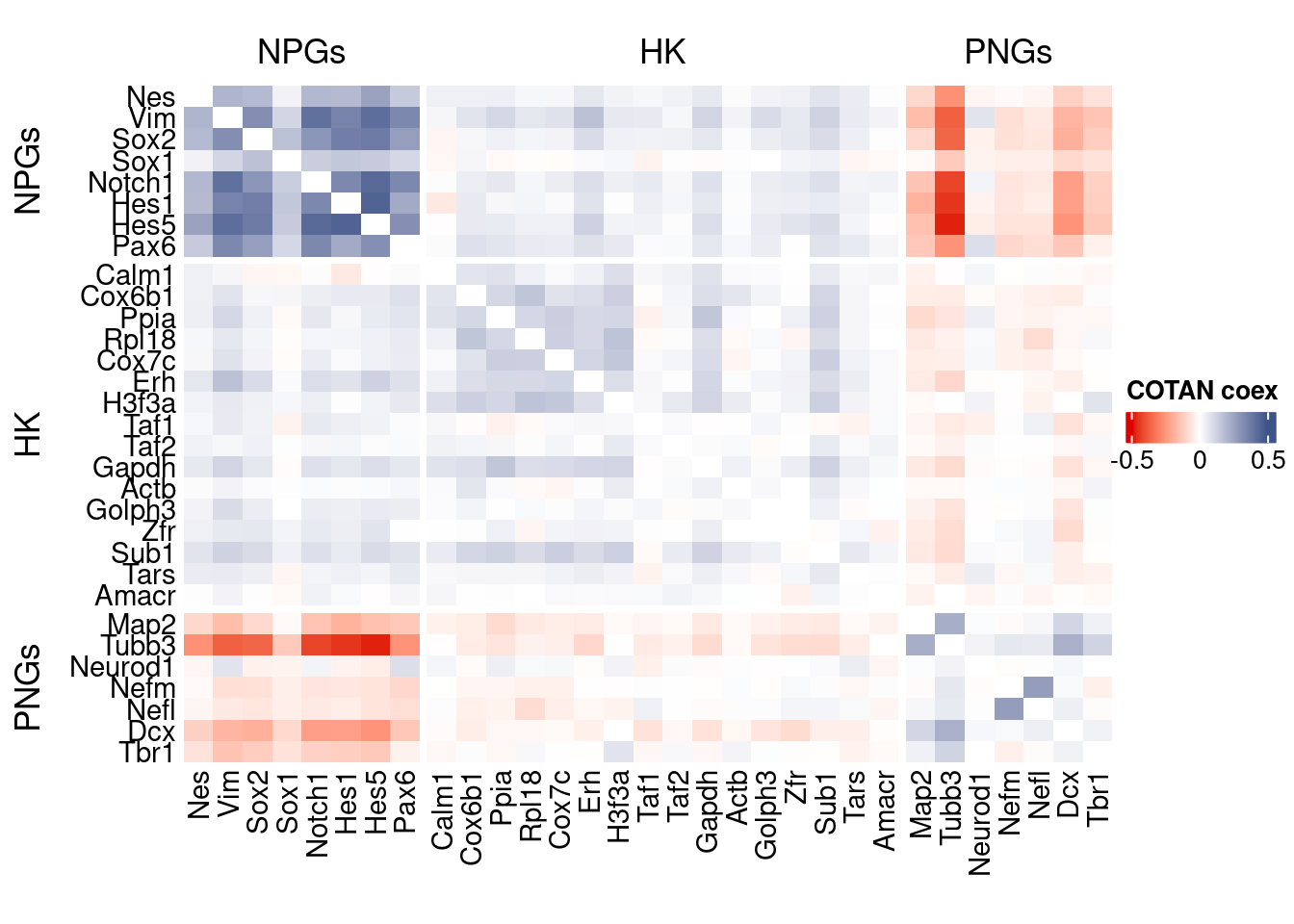
GDI_DF <- calculateGDI(obj)
GDI_DF$geneType <- NA
for (cat in names(genesList)) {
  GDI_DF[rownames(GDI_DF) %in% genesList[[cat]],]$geneType <- cat
}

GDI_DF$GDI_centered <- scale(GDI_DF$GDI,center = T,scale = T)

GDI_DF[genesFromListExpressed,]
sum.raw.norm GDI exp.cells geneType GDI_centered
Nes 5.354860 2.677591 7.6611269 NPGs 2.12164684
Vim 7.975351 3.653910 23.7130118 NPGs 4.21500654
Sox2 5.379522 3.446151 6.6477503 NPGs 3.76954465
Sox1 4.826847 2.321489 3.8913660 NPGs 1.35811585
Notch1 5.491804 3.644973 8.1070126 NPGs 4.19584566
Hes1 5.241888 3.715489 4.4183218 NPGs 4.34704054
Hes5 6.367234 3.706690 6.9720308 NPGs 4.32817408
Pax6 6.445184 3.410841 15.2006486 NPGs 3.69383388
Map2 8.945220 2.919301 87.3530604 PNGs 2.63990577
Tubb3 10.669909 3.802683 93.9602756 PNGs 4.53399718
Neurod1 4.512176 1.570675 3.2833401 PNGs -0.25172970
Nefm 5.320286 2.010487 6.2829347 PNGs 0.69128553
Nefl 5.592561 2.179108 5.2695582 PNGs 1.05283171
Dcx 8.048568 2.850882 60.6404540 PNGs 2.49320624
Tbr1 6.829413 1.953272 23.6724767 PNGs 0.56860885
Calm1 9.893664 1.604866 97.6489664 hk -0.17841926
Cox6b1 9.028070 2.184997 90.8796109 hk 1.06545895
Ppia 9.189622 2.372214 90.7580057 hk 1.46687705
Rpl18 9.554798 2.279009 96.3518443 hk 1.26703311
Cox7c 9.114185 2.170535 91.9740576 hk 1.03444998
Erh 7.929830 2.390307 62.5050669 hk 1.50567107
H3f3a 9.697620 2.349951 96.3518443 hk 1.41914319
Taf1 6.206264 1.475777 16.9436563 hk -0.45520422
Taf2 5.648276 1.342082 10.2959060 hk -0.74186428
Gapdh 8.621629 2.367727 80.5026348 hk 1.45725765
Actb 10.484376 1.292044 99.6351844 hk -0.84915323
Golph3 5.947435 1.643738 13.8629915 hk -0.09507358
Zfr 7.359818 1.675085 43.6157276 hk -0.02786120
Sub1 8.434336 2.419785 75.3952169 hk 1.56887719
Tars 5.930970 1.571117 13.5387110 hk -0.25078126
Amacr 4.339515 1.454028 2.9995946 hk -0.50183660
Reln 6.723819 2.232753 4.7020673 layers 1.16785364
Lhx5 4.079754 2.579243 1.3376571 layers 1.91077584
Cux1 7.968038 2.190834 50.0202675 layers 1.07797409
Satb2 9.062287 3.390857 57.7219295 layers 3.65098593
Tle1 6.594351 1.618541 21.7673287 layers -0.14909808
Mef2c 9.071730 3.175241 51.6011350 layers 3.18867667
Rorb 6.282362 1.926899 13.1333604 layers 0.51206224
Sox5 8.049776 2.285548 43.4130523 layers 1.28105506
Bcl11b 7.109492 2.116159 21.4835833 layers 0.91786051
Fezf2 6.506386 2.096344 18.1597081 layers 0.87537638
Foxp2 6.557695 2.455294 14.4304824 layers 1.64501202
Ntf3 6.051423 2.225961 6.9314957 layers 1.15329231
Rasgrf2 4.096064 1.795794 2.0267531 layers 0.23095491
Cux2 7.067401 2.518402 26.4288610 layers 1.78032434
Slc17a6 6.228895 2.065176 14.4304824 layers 0.80854728
Sema3c 7.553723 2.676192 31.6984191 layers 2.11864837
Thsd7a 5.951856 1.810789 9.6068099 layers 0.26310666
Sulf2 4.348066 1.725374 2.3915687 layers 0.07996546
Kcnk2 7.512577 1.895654 41.7511147 layers 0.44506877
Grik3 5.173332 1.974505 4.4993920 layers 0.61413535
Etv1 5.383398 2.639083 5.8775841 layers 2.03908090
Tle4 5.664300 1.881239 8.4718281 layers 0.41416114
Tmem200a 5.235004 2.081666 6.3234698 layers 0.84390268
Glra2 6.076633 2.094562 11.2687475 layers 0.87155349
Etv1.1 5.383398 2.639083 5.8775841 layers 2.03908090
Htr1f 3.780477 1.777503 1.2160519 layers 0.19173786
Sulf1 2.631257 1.128008 0.3648156 layers -1.20086709
Syt6 4.757520 1.609693 2.6347791 layers -0.16807098GDIPlot(obj,GDIIn = GDI_DF, genes = genesList,GDIThreshold = 1.4)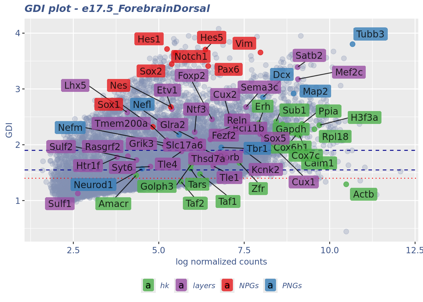
Seurat correlation
srat<- CreateSeuratObject(counts = getRawData(obj),
                          project = project,
                          min.cells = 3,
                          min.features = 200)
srat[["percent.mt"]] <- PercentageFeatureSet(srat, pattern = "^mt-")
srat <- NormalizeData(srat)
srat <- FindVariableFeatures(srat, selection.method = "vst", nfeatures = 2000)

# plot variable features with and without labels
plot1 <- VariableFeaturePlot(srat)

plot1$data$centered_variance <- scale(plot1$data$variance.standardized,
                                      center = T,scale = F)

write.csv(plot1$data,paste0("CoexData/",
                            "Variance_Seurat_genes",
                            getMetadataElement(obj,
                                               datasetTags()[["cond"]]),".csv"))

LabelPoints(plot = plot1, points = c(genesList$NPGs,genesList$PNGs,genesList$layers), repel = TRUE)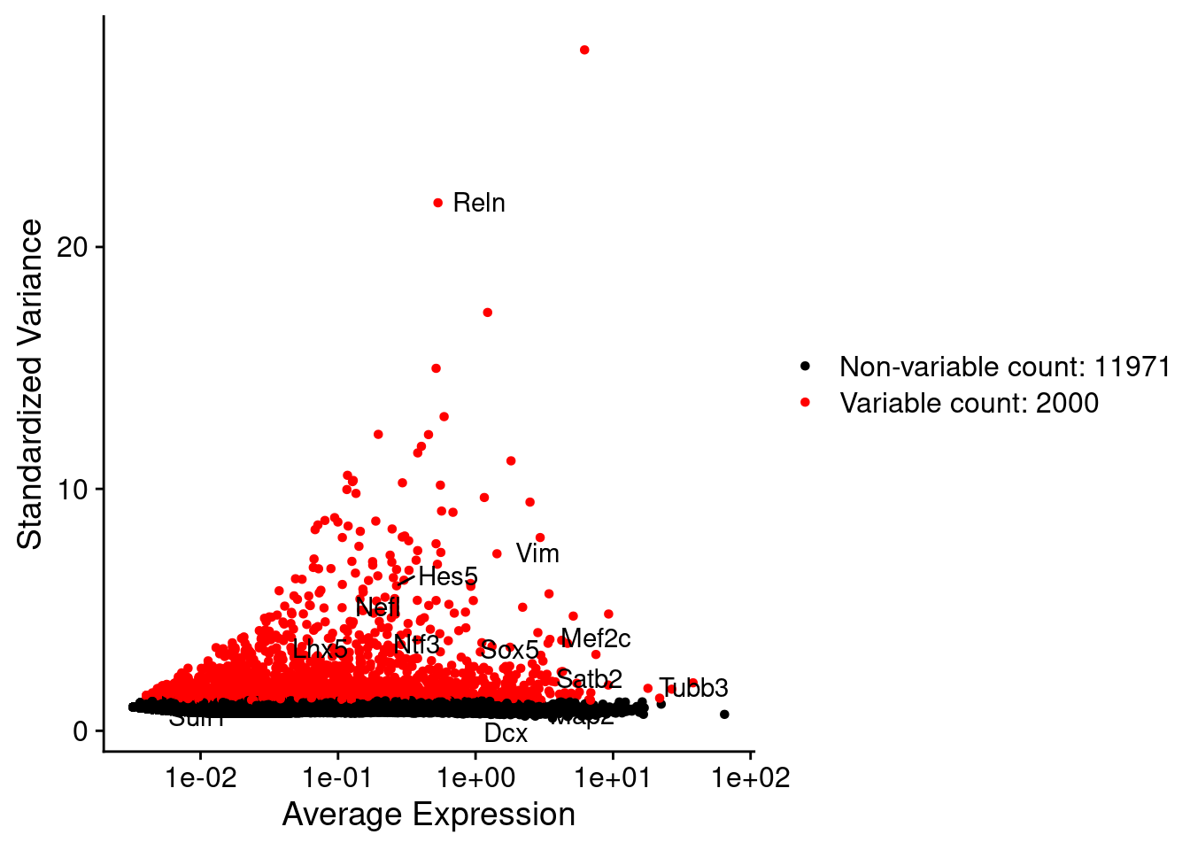
LabelPoints(plot = plot1, points = c(genesList$hk), repel = TRUE)
all.genes <- rownames(srat)
srat <- ScaleData(srat, features = all.genes)
seurat.data = GetAssayData(srat[["RNA"]],layer = "data")
corr.pval.list <- correlation_pvalues(data = seurat.data,
genesFromListExpressed,
n.cells = getNumCells(obj))
seurat.data.cor.big <- as.matrix(Matrix::forceSymmetric(corr.pval.list$data.cor, uplo = "U"))
htmp <- correlation_plot(seurat.data.cor.big,
genesList, title="Seurat corr")
p_values.fromSeurat <- corr.pval.list$p_values
seurat.data.cor.big <- corr.pval.list$data.cor
rm(corr.pval.list)
gc() used (Mb) gc trigger (Mb) max used (Mb)
Ncells 10157451 542.5 17749782 948.0 17749782 948.0
Vcells 186033678 1419.4 597867832 4561.4 746885213 5698.3draw(htmp, heatmap_legend_side="right")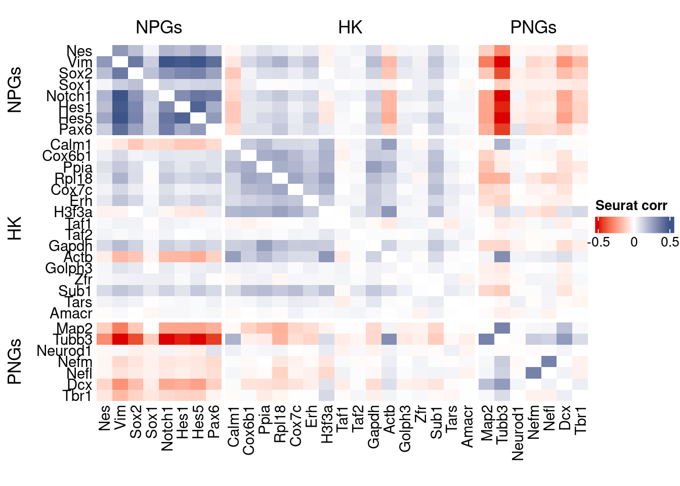
rm(seurat.data.cor.big)
rm(p_values.fromSeurat)
Seurat SC Transform
srat <-  SCTransform(srat,
                     method = "glmGamPoi",
                     vars.to.regress = "percent.mt",
                     verbose = FALSE)

seurat.data <- GetAssayData(srat[["SCT"]],layer = "data")

#Remove genes with all zeros
seurat.data <-seurat.data[rowSums(seurat.data) > 0,]


corr.pval.list <- correlation_pvalues(seurat.data,
                                      genesFromListExpressed,
                                      n.cells = getNumCells(obj))


seurat.data.cor.big <- as.matrix(Matrix::forceSymmetric(corr.pval.list$data.cor, uplo = "U"))

htmp <- correlation_plot(seurat.data.cor.big,
                         genesList, title="Seurat corr SCT")


p_values.fromSeurat <- corr.pval.list$p_values
seurat.data.cor.big <- corr.pval.list$data.cor

rm(corr.pval.list)
gc()
used (Mb) gc trigger (Mb) max used (Mb)
Ncells 10485956 560.1 17749782 948.0 17749782 948.0
Vcells 209299091 1596.9 597867832 4561.4 746885213 5698.3draw(htmp, heatmap_legend_side="right")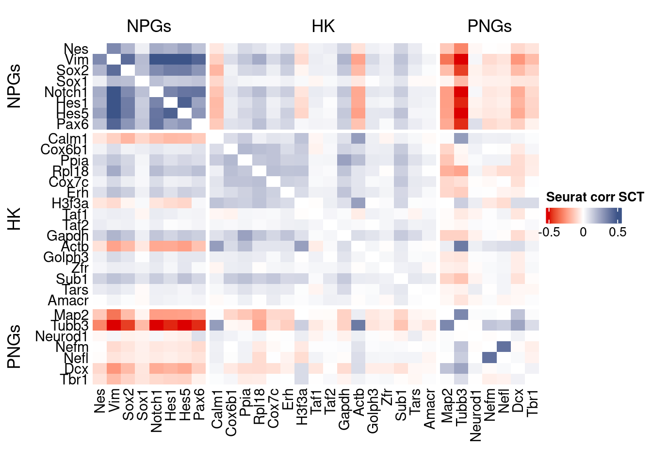
plot1 <- VariableFeaturePlot(srat)

plot1$data$centered_variance <- scale(plot1$data$residual_variance,
center = T,scale = F)write.csv(plot1$data,paste0("CoexData/",
"Variance_SeuratSCT_genes",
getMetadataElement(obj,
datasetTags()[["cond"]]),".csv"))
write_fst(as.data.frame(seurat.data.cor.big),path = paste0("CoexData/SeuratCorrSCT_",file_code,".fst"), compress = 100)
write_fst(as.data.frame(p_values.fromSeurat),path = paste0("CoexData/SeuratPValuesSCT_", file_code,".fst"))
write.csv(as.data.frame(p_values.fromSeurat),paste0("CoexData/SeuratPValuesSCT_", file_code,".csv"))
rm(seurat.data.cor.big)
rm(p_values.fromSeurat)Monocle
library(monocle3)cds <- new_cell_data_set(getRawData(obj),
cell_metadata = getMetadataCells(obj),
gene_metadata = getMetadataGenes(obj)
)
cds <- preprocess_cds(cds, num_dim = 100)
normalized_counts <- normalized_counts(cds)#Remove genes with all zeros
normalized_counts <- normalized_counts[rowSums(normalized_counts) > 0,]
corr.pval.list <- correlation_pvalues(normalized_counts,
genesFromListExpressed,
n.cells = getNumCells(obj))
rm(normalized_counts)
monocle.data.cor.big <- as.matrix(Matrix::forceSymmetric(corr.pval.list$data.cor, uplo = "U"))
htmp <- correlation_plot(data.cor.big = monocle.data.cor.big,
genesList,
title = "Monocle corr")
p_values.from.monocle <- corr.pval.list$p_values
monocle.data.cor.big <- corr.pval.list$data.cor
rm(corr.pval.list)
gc() used (Mb) gc trigger (Mb) max used (Mb)
Ncells 10672221 570.0 17749782 948.0 17749782 948.0
Vcells 211297760 1612.1 597867832 4561.4 746885213 5698.3draw(htmp, heatmap_legend_side="right")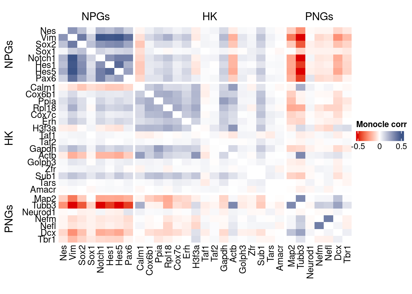
ScanPy
library(reticulate)

dirOutScP <- paste0("CoexData/ScanPy/")
if (!dir.exists(dirOutScP)) {
  dir.create(dirOutScP)
}
if(Sys.info()[["sysname"]] == "Windows"){

  use_python("C:/Users/Silvia/miniconda3/envs/r-scanpy/python.exe", required = TRUE)
  #Sys.setenv(RETICULATE_PYTHON = "C:/Users/Silvia/AppData/Local/Python/pythoncore-3.14-64/python.exe" )
}else{
  Sys.setenv(RETICULATE_PYTHON = "../../../bin/python3")
}

  py <- import("sys")

  source_python("src/scanpyGenesExpression.py")
  scanpyFDR(getRawData(obj),
                  getMetadataCells(obj),
                  getMetadataGenes(obj),
                   "mt",
                   dirOutScP,
                   file_code,
            int.genes)
inizio
open pdfnormalized_counts <- read.csv(paste0(dirOutScP,
file_code,"_Scanpy_expression_all_genes.gz"),header = T,row.names = 1)
normalized_counts <- t(normalized_counts)#Remove genes with all zeros
normalized_counts <-normalized_counts[rowSums(normalized_counts) > 0,]
corr.pval.list <- correlation_pvalues(normalized_counts,
genesFromListExpressed,
n.cells = getNumCells(obj))
ScanPy.data.cor.big <- as.matrix(Matrix::forceSymmetric(corr.pval.list$data.cor, uplo = "U"))
htmp <- correlation_plot(data.cor.big = ScanPy.data.cor.big,
genesList,
title = "ScanPy corr")
p_values.from.ScanPy <- corr.pval.list$p_values
ScanPy.data.cor.big <- corr.pval.list$data.cor
rm(corr.pval.list)
gc() used (Mb) gc trigger (Mb) max used (Mb)
Ncells 10693003 571.1 17749782 948.0 17749782 948.0
Vcells 253633520 1935.1 597867832 4561.4 746885213 5698.3draw(htmp, heatmap_legend_side="right")
Cs-Core
library(CSCORE)Convert to Seurat obj
sceObj <- convertToSingleCellExperiment(obj)

# Correct: assay=NULL (or omit), data=NULL (since no logcounts)
seuratObj <- as.Seurat(
  x       = sceObj,
  counts  = "counts",
  data    = NULL,
  assay   = NULL,      # IMPORTANT: do NOT set to "RNA" here
  project = "COTAN"
)

# as.Seurat(SCE) creates assay "originalexp" by default; rename it to RNA
seuratObj <- RenameAssays(seuratObj, originalexp = "RNA", verbose = FALSE)
DefaultAssay(seuratObj) <- "RNA"

# Optional: keep COTAN payload
seuratObj@misc$COTAN <- S4Vectors::metadata(sceObj)
Extract CS_CORE corr matrix
#seuratObj@assays$RNA@counts <- ceiling(seuratObj@assays$RNA@counts)
csCoreRes <- CSCORE(seuratObj, genes = genesFromListExpressed)
[INFO] IRLS converged after 3 iterations.
[INFO] Starting WLS for covariance at Thu Jan 22 14:16:49 2026
[INFO] 0.0584% co-expression estimates were greater than 1 and were set to 1.
[INFO] 0.0000% co-expression estimates were smaller than -1 and were set to -1.
[INFO] Finished WLS. Elapsed time: 0.0600 seconds.mat <- as.matrix(csCoreRes$est)
diag(mat) <- 0
split.genes <- base::factor(c(rep("NPGs",sum(genesList[["NPGs"]] %in% genesFromListExpressed)),
rep("HK",sum(genesList[["hk"]] %in% genesFromListExpressed)),
rep("PNGs",sum(genesList[["PNGs"]] %in% genesFromListExpressed))
),
levels = c("NPGs","HK","PNGs"))
f1 = colorRamp2(seq(-0.5,0.5, length = 3), c("#DC0000B2", "white","#3C5488B2" ))
htmp <- Heatmap(as.matrix(mat[c(genesList$NPGs,genesList$hk,genesList$PNGs),c(genesList$NPGs,genesList$hk,genesList$PNGs)]),
#width = ncol(coexMat)*unit(2.5, "mm"),
height = nrow(mat)*unit(3, "mm"),
cluster_rows = FALSE,
cluster_columns = FALSE,
col = f1,
row_names_side = "left",
row_names_gp = gpar(fontsize = 11),
column_names_gp = gpar(fontsize = 11),
column_split = split.genes,
row_split = split.genes,
cluster_row_slices = FALSE,
cluster_column_slices = FALSE,
heatmap_legend_param = list(
title = "CS-CORE", at = c(-0.5, 0, 0.5),
direction = "horizontal",
labels = c("-0.5", "0", "0.5")
)
)
draw(htmp, heatmap_legend_side="right")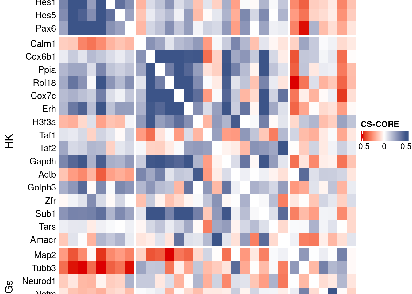
Save CS_CORE matrix
write_fst(as.data.frame(csCoreRes$est), path = paste0("CoexData/CS_CORECorr_", file_code,".fst"),compress = 100)
write_fst(as.data.frame(csCoreRes$p_value), path = paste0("CoexData/CS_COREPValues_", file_code,".fst"),compress = 100)
write.csv(as.data.frame(csCoreRes$p_value), paste0("CoexData/CS_COREPValues_", file_code,".csv"))
Baseline: Spearman on UMI counts
corr.pval.list <- correlation_pvaluesSpearman(data = getRawData(obj),
                                      genesFromListExpressed,
                                      n.cells = getNumCells(obj))

data.cor.big <- as.matrix(Matrix::forceSymmetric(corr.pval.list$data.cor, uplo = "U"))

htmp <- correlation_plot(data.cor.big,
                         genesList, title="UMI baseline S. corr")


p_values.fromSp.C <- corr.pval.list$p_values
data.cor.bigSp.C <- corr.pval.list$data.cor

rm(corr.pval.list)
gc()
used (Mb) gc trigger (Mb) max used (Mb)
Ncells 10701317 571.6 17749782 948.0 17749782 948.0
Vcells 246028507 1877.1 597867832 4561.4 746885213 5698.3draw(htmp, heatmap_legend_side="right")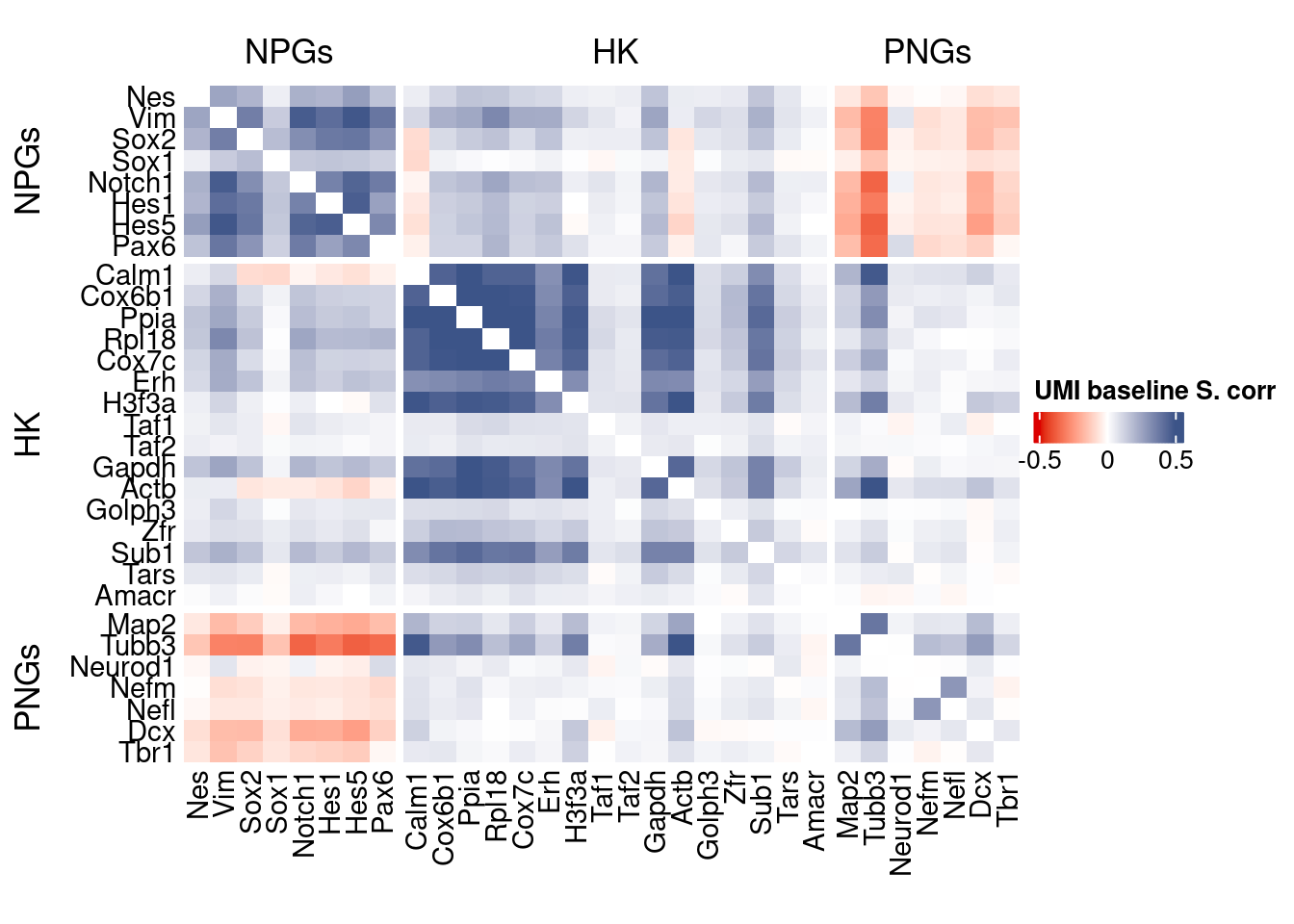
write.csv(as.data.frame(p_values.fromSp.C), paste0("CoexData/BaselineUMISpCorrPValues_", file_code,".csv"))Baseline: Pearson on binarized counts
corr.pval.list <- correlation_pvalues(data = getZeroOneProj(obj),
                                      genesFromListExpressed,
                                      n.cells = getNumCells(obj))

data.cor.big <- as.matrix(Matrix::forceSymmetric(corr.pval.list$data.cor, uplo = "U"))

htmp <- correlation_plot(data.cor.big,
                         genesList, title="Zero-one P. corr")


p_values.fromSp.C <- corr.pval.list$p_values
data.cor.bigSp.C <- corr.pval.list$data.cor

rm(corr.pval.list)
gc()
used (Mb) gc trigger (Mb) max used (Mb)
Ncells 10701450 571.6 17749782 948.0 17749782 948.0
Vcells 246028774 1877.1 597867832 4561.4 746885213 5698.3draw(htmp, heatmap_legend_side="right")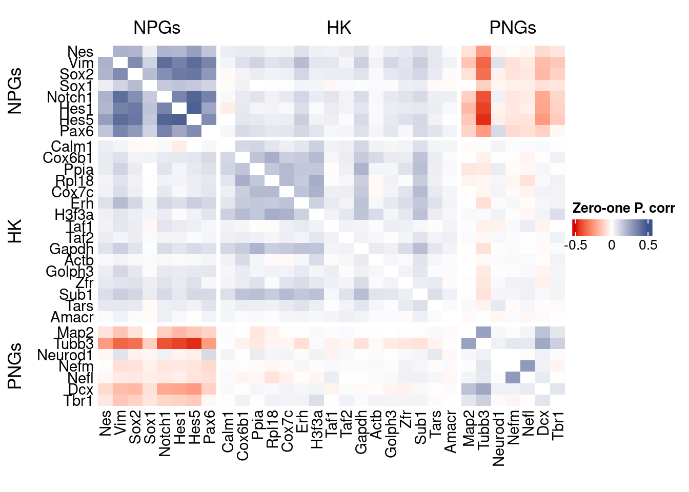
write.csv(as.data.frame(p_values.fromSp.C), paste0("CoexData/ZeroOnePCorrPValues_", file_code,".csv"))Sys.time()[1] "2026-01-22 14:16:53 CET"sessionInfo()R version 4.5.2 (2025-10-31)
Platform: x86_64-pc-linux-gnu
Running under: Ubuntu 22.04.5 LTS
Matrix products: default
BLAS: /usr/lib/x86_64-linux-gnu/blas/libblas.so.3.10.0
LAPACK: /usr/lib/x86_64-linux-gnu/lapack/liblapack.so.3.10.0 LAPACK version 3.10.0
locale:
[1] LC_CTYPE=C.UTF-8 LC_NUMERIC=C LC_TIME=C.UTF-8
[4] LC_COLLATE=C.UTF-8 LC_MONETARY=C.UTF-8 LC_MESSAGES=C.UTF-8
[7] LC_PAPER=C.UTF-8 LC_NAME=C LC_ADDRESS=C
[10] LC_TELEPHONE=C LC_MEASUREMENT=C.UTF-8 LC_IDENTIFICATION=C
time zone: Europe/Rome
tzcode source: system (glibc)
attached base packages:
[1] stats4 parallel grid stats graphics grDevices utils
[8] datasets methods base
other attached packages:
[1] CSCORE_1.0.2 reticulate_1.44.1
[3] monocle3_1.3.7 SingleCellExperiment_1.32.0
[5] SummarizedExperiment_1.38.1 GenomicRanges_1.62.1
[7] Seqinfo_1.0.0 IRanges_2.44.0
[9] S4Vectors_0.48.0 MatrixGenerics_1.22.0
[11] matrixStats_1.5.0 Biobase_2.70.0
[13] BiocGenerics_0.56.0 generics_0.1.3
[15] fstcore_0.10.0 fst_0.9.8
[17] stringr_1.6.0 HiClimR_2.2.1
[19] doParallel_1.0.17 iterators_1.0.14
[21] foreach_1.5.2 Rfast_2.1.5.1
[23] RcppParallel_5.1.10 zigg_0.0.2
[25] Rcpp_1.1.0 patchwork_1.3.2
[27] Seurat_5.4.0 SeuratObject_5.3.0
[29] sp_2.2-0 Hmisc_5.2-3
[31] dplyr_1.1.4 circlize_0.4.16
[33] ComplexHeatmap_2.26.0 COTAN_2.11.1
loaded via a namespace (and not attached):
[1] RcppAnnoy_0.0.22 splines_4.5.2
[3] later_1.4.2 tibble_3.3.0
[5] polyclip_1.10-7 rpart_4.1.24
[7] fastDummies_1.7.5 lifecycle_1.0.4
[9] Rdpack_2.6.4 globals_0.18.0
[11] lattice_0.22-7 MASS_7.3-65
[13] backports_1.5.0 ggdist_3.3.3
[15] dendextend_1.19.0 magrittr_2.0.4
[17] plotly_4.11.0 rmarkdown_2.29
[19] yaml_2.3.10 httpuv_1.6.16
[21] otel_0.2.0 glmGamPoi_1.20.0
[23] sctransform_0.4.2 spam_2.11-1
[25] spatstat.sparse_3.1-0 minqa_1.2.8
[27] cowplot_1.2.0 pbapply_1.7-2
[29] RColorBrewer_1.1-3 abind_1.4-8
[31] Rtsne_0.17 purrr_1.2.0
[33] nnet_7.3-20 GenomeInfoDbData_1.2.14
[35] ggrepel_0.9.6 irlba_2.3.5.1
[37] listenv_0.10.0 spatstat.utils_3.2-1
[39] goftest_1.2-3 RSpectra_0.16-2
[41] spatstat.random_3.4-3 fitdistrplus_1.2-2
[43] parallelly_1.46.0 DelayedMatrixStats_1.30.0
[45] ncdf4_1.24 codetools_0.2-20
[47] DelayedArray_0.36.0 tidyselect_1.2.1
[49] shape_1.4.6.1 UCSC.utils_1.4.0
[51] farver_2.1.2 lme4_1.1-37
[53] ScaledMatrix_1.16.0 viridis_0.6.5
[55] base64enc_0.1-3 spatstat.explore_3.6-0
[57] jsonlite_2.0.0 GetoptLong_1.1.0
[59] Formula_1.2-5 progressr_0.18.0
[61] ggridges_0.5.6 survival_3.8-3
[63] tools_4.5.2 ica_1.0-3
[65] glue_1.8.0 gridExtra_2.3
[67] SparseArray_1.10.8 xfun_0.52
[69] distributional_0.6.0 ggthemes_5.2.0
[71] GenomeInfoDb_1.44.0 withr_3.0.2
[73] fastmap_1.2.0 boot_1.3-32
[75] digest_0.6.37 rsvd_1.0.5
[77] parallelDist_0.2.6 R6_2.6.1
[79] mime_0.13 colorspace_2.1-1
[81] Cairo_1.7-0 scattermore_1.2
[83] tensor_1.5 spatstat.data_3.1-9
[85] tidyr_1.3.1 data.table_1.18.0
[87] httr_1.4.7 htmlwidgets_1.6.4
[89] S4Arrays_1.10.1 uwot_0.2.3
[91] pkgconfig_2.0.3 gtable_0.3.6
[93] lmtest_0.9-40 S7_0.2.1
[95] XVector_0.50.0 htmltools_0.5.8.1
[97] dotCall64_1.2 clue_0.3-66
[99] scales_1.4.0 png_0.1-8
[101] reformulas_0.4.1 spatstat.univar_3.1-6
[103] rstudioapi_0.18.0 knitr_1.50
[105] reshape2_1.4.4 rjson_0.2.23
[107] nloptr_2.2.1 checkmate_2.3.2
[109] nlme_3.1-168 proxy_0.4-29
[111] zoo_1.8-14 GlobalOptions_0.1.2
[113] KernSmooth_2.23-26 miniUI_0.1.2
[115] foreign_0.8-90 pillar_1.11.1
[117] vctrs_0.7.0 RANN_2.6.2
[119] promises_1.5.0 BiocSingular_1.26.1
[121] beachmat_2.26.0 xtable_1.8-4
[123] cluster_2.1.8.1 htmlTable_2.4.3
[125] evaluate_1.0.5 magick_2.9.0
[127] zeallot_0.2.0 cli_3.6.5
[129] compiler_4.5.2 rlang_1.1.7
[131] crayon_1.5.3 future.apply_1.20.0
[133] labeling_0.4.3 plyr_1.8.9
[135] stringi_1.8.7 viridisLite_0.4.2
[137] deldir_2.0-4 BiocParallel_1.44.0
[139] assertthat_0.2.1 lazyeval_0.2.2
[141] spatstat.geom_3.6-1 Matrix_1.7-4
[143] RcppHNSW_0.6.0 sparseMatrixStats_1.20.0
[145] future_1.69.0 ggplot2_4.0.1
[147] shiny_1.12.1 rbibutils_2.3
[149] ROCR_1.0-11 igraph_2.2.1