library (ggplot2)library (tibble)library (zeallot)library (COTAN)library (plyr)library (scales) library (rlang)library (Seurat)library (wordcloud)library (stringr)library (assertr)library (ggVennDiagram)library (ggplot2)library (tidyr)library (enrichR)<- getOption ("enrichR.live" )if (websiteLive) dbs <- listEnrichrDbs ()head (dbs)
  geneCoverage genesPerTerm                      libraryName
1        13362          275              Genome_Browser_PWMs
2        27884         1284         TRANSFAC_and_JASPAR_PWMs
3         6002           77        Transcription_Factor_PPIs
4        47172         1370                        ChEA_2013
5        47107          509 Drug_Perturbations_from_GEO_2014
6        21493         3713          ENCODE_TF_ChIP-seq_2014
                                                      link numTerms
1 http://hgdownload.cse.ucsc.edu/goldenPath/hg18/database/      615
2                 http://jaspar.genereg.net/html/DOWNLOAD/      326
3                                                               290
4           http://amp.pharm.mssm.edu/lib/cheadownload.jsp      353
5                         http://www.ncbi.nlm.nih.gov/geo/      701
6             http://genome.ucsc.edu/ENCODE/downloads.html      498
                                   appyter categoryId
1 ea115789fcbf12797fd692cec6df0ab4dbc79c6a          1
2 7d42eb43a64a4e3b20d721fc7148f685b53b6b30          1
3 849f222220618e2599d925b6b51868cf1dab3763          1
4 7ebe772afb55b63b41b79dd8d06ea0fdd9fa2630          7
5 ad270a6876534b7cb063e004289dcd4d3164f342          7
6 497787ebc418d308045efb63b8586f10c526af51          7
#dbs <- "Tabula_Muris" <- "ARCHS4_Tissues" options (parallelly.fork.enable = TRUE )<- "./e15.0_FD_CheckClustersUniformity" setLoggingLevel (1 )setLoggingFile (file.path (outDir, "FindUniformGivenClustersInForebrainDorsal_E150.log" ))
<- readRDS (file = file.path ("Data/MouseCortexFromLoom/SourceData/" , "e15.0_ForebrainDorsal.cotan.RDS" ))<- readRDS (file = file.path ("Data/MouseCortexFromLoom/" , "e15.0_ForebrainDorsal.cotan.RDS" ))
Align to cleaned cells’ list
<- getMetadataCells (fb150ObjRaw)[getCells (fb150Obj), ]#metaCDrop <- getMetadataCells(fb150ObjRaw)[!getCells(fb150ObjRaw) %in% getCells(fb150Obj), ]
Extract the cells of class ‘Neuron’
<- metaC[metaC[["Class" ]] == "Neuron" , ]sort (table (metaNeuron[["Subclass" ]]), decreasing = TRUE )
Cortical or hippocampal glutamatergic                   Forebrain GABAergic
                                 3969                                   610
                        Cajal-Retzius                Mixed region GABAergic
                                  145                                    21
                            Undefined               Forebrain glutamatergic
                                   16                                    15
                         Hypothalamus            Mixed region glutamatergic
                                    8                                     5
    Mixed region and neurotransmitter               Hindbrain glutamatergic
                                    4                                     2
                Hindbrain glycinergic            Hypothalamus glutamatergic
                                    2                                     2
        Dorsal midbrain glutamatergic                          Mixed region
                                    1                                     1
sort (table (metaNeuron[["ClusterName" ]]), decreasing = TRUE )
Neur525 Neur511 Neur509 Neur510 Neur508 Neur507 Neur568 Neur504 Neur505 Neur516
    826     540     402     402     397     183     181     174     147     137
Neur565 Neur524 Neur679 Neur493 Neur498 Neur497 Neur506 Neur502 Neur494 Neur574
    133     108     105      93      79      51      46      42      41      41
Neur575 Neur492 Neur519 Neur526 Neur566 Neur501 Neur573 Neur499 Neur518 Neur560
     41      38      31      28      28      24      24      23      22      20
Neur514 Neur523 Neur569 Neur557 Neur495 Neur520 Neur535 Neur542 Neur677 Neur527
     19      19      18      16      15      15      14      14      14      13
Neur496 Neur512 Neur676 Neur517 Neur558 Neur503 Neur739 Neur559 Neur564 Neur538
     11      11      11      10       9       8       8       7       7       6
Neur549 Neur561 Neur671 Neur695 Neur738 Neur747 Neur500 Neur536 Neur678 Neur534
      6       6       6       6       6       6       5       5       5       4
Neur550 Neur570 Neur686 Neur731 Neur737 Neur513 Neur515 Neur528 Neur533 Neur539
      4       4       4       4       4       3       3       3       3       3
Neur544 Neur571 Neur674 Neur675 Neur732 Neur531 Neur543 Neur548 Neur552 Neur554
      3       3       3       3       3       2       2       2       2       2
Neur562 Neur670 Neur689 Neur740 Neur529 Neur530 Neur532 Neur537 Neur540 Neur553
      2       2       2       2       1       1       1       1       1       1
Neur567 Neur572 Neur601 Neur614 Neur634 Neur647 Neur649 Neur672 Neur680 Neur681
      1       1       1       1       1       1       1       1       1       1
Neur684 Neur693 Neur696 Neur726 Neur734 Neur749 Neur750 Neur751 Neur760 Neur771
      1       1       1       1       1       1       1       1       1       1
<- names (table (metaNeuron[["ClusterName" ]])[table (metaNeuron[["ClusterName" ]]) >= 20L])<- metaNeuron[metaNeuron$ ClusterName %in% cl.to.keep,]dim (meta.to.keep)
Dropped cell
dim (metaNeuron)[1 ] - dim (meta.to.keep)[1 ]
Removing cells
<- getCells (fb150Obj)[! getCells (fb150Obj) %in% rownames (meta.to.keep)]<- dropGenesCells (fb150Obj,cells = cell.to.drop)dim (meta.to.keep)[1 ] == dim (getRawData (fb150Obj))[2 ]<- getMetadataCells (fb150ObjRaw)[getCells (fb150Obj), ]
<- clean (fb150Obj)<- estimateDispersionBisection (fb150Obj)identical (rownames (fb150Obj@ metaCells), rownames (metaC))@ metaCells <- cbind (fb150Obj@ metaCells,metaC)@ metaCells[1 : 10 ,]
                            feCells        nu feCells        nu   Age
10X74_4_A_1:TGGTAGACCCTACCx   FALSE 0.9375770   FALSE 0.9214807 e15.0
10X73_3_A_1:TACCGGCTTCAGTGx   FALSE 0.7855991   FALSE 0.7722440 e15.0
10X74_4_A_1:CCCAGTTGGAGGTGx   FALSE 0.6983103   FALSE 0.6863260 e15.0
10X73_3_A_1:AATTGATGAGAATGx   FALSE 1.1751850   FALSE 1.1548031 e15.0
10X74_4_A_1:TAGTGGTGAGTAGAx   FALSE 1.1001290   FALSE 1.0808973 e15.0
10X74_4_A_1:ATTATGGACTACGAx   FALSE 1.3074658   FALSE 1.2844945 e15.0
10X64_3_A_1:TGTATCTGCCTTATx   FALSE 1.4138296   FALSE 1.3891434 e15.0
10X64_3_A_1:TAGTATGACTATGGx   FALSE 1.6528889   FALSE 1.6249089 e15.0
10X73_3_A_1:ACTTGGGATTGCAGx   FALSE 0.7482785   FALSE 0.7355965 e15.0
10X74_4_A_1:AGCTCGCTCCATGAx   FALSE 1.1109106   FALSE 1.0914844 e15.0
                                       CellCycle                      CellID
10X74_4_A_1:TGGTAGACCCTACCx  0.00308982564555286 10X74_4_A_1:TGGTAGACCCTACCx
10X73_3_A_1:TACCGGCTTCAGTGx 0.000789058390320884 10X73_3_A_1:TACCGGCTTCAGTGx
10X74_4_A_1:CCCAGTTGGAGGTGx  0.00177988727380599 10X74_4_A_1:CCCAGTTGGAGGTGx
10X73_3_A_1:AATTGATGAGAATGx 0.000880436696601514 10X73_3_A_1:AATTGATGAGAATGx
10X74_4_A_1:TAGTGGTGAGTAGAx 0.000752021056589585 10X74_4_A_1:TAGTGGTGAGTAGAx
10X74_4_A_1:ATTATGGACTACGAx  0.00174133291119202 10X74_4_A_1:ATTATGGACTACGAx
10X64_3_A_1:TGTATCTGCCTTATx 0.000878348704435661 10X64_3_A_1:TGTATCTGCCTTATx
10X64_3_A_1:TAGTATGACTATGGx  0.00125156445556946 10X64_3_A_1:TAGTATGACTATGGx
10X73_3_A_1:ACTTGGGATTGCAGx  0.00221177771633951 10X73_3_A_1:ACTTGGGATTGCAGx
10X74_4_A_1:AGCTCGCTCCATGAx  0.00111835973904939 10X74_4_A_1:AGCTCGCTCCATGAx
                            Cell_Conc Chemistry ChipID  Class ClusterName
10X74_4_A_1:TGGTAGACCCTACCx       600        v2  10X74 Neuron     Neur492
10X73_3_A_1:TACCGGCTTCAGTGx       600        v2  10X73 Neuron     Neur492
10X74_4_A_1:CCCAGTTGGAGGTGx       600        v2  10X74 Neuron     Neur492
10X73_3_A_1:AATTGATGAGAATGx       600        v2  10X73 Neuron     Neur492
10X74_4_A_1:TAGTGGTGAGTAGAx       600        v2  10X74 Neuron     Neur492
10X74_4_A_1:ATTATGGACTACGAx       600        v2  10X74 Neuron     Neur492
10X64_3_A_1:TGTATCTGCCTTATx       600        v2  10X64 Neuron     Neur492
10X64_3_A_1:TAGTATGACTATGGx       600        v2  10X64 Neuron     Neur492
10X73_3_A_1:ACTTGGGATTGCAGx       600        v2  10X73 Neuron     Neur492
10X74_4_A_1:AGCTCGCTCCATGAx       600        v2  10X74 Neuron     Neur492
                            Clusters Date_Captured    DonorID
10X74_4_A_1:TGGTAGACCCTACCx      492    2016-11-30 Batch14K-2
10X73_3_A_1:TACCGGCTTCAGTGx      492    2016-11-30 Batch14K-2
10X74_4_A_1:CCCAGTTGGAGGTGx      492    2016-11-30 Batch14K-2
10X73_3_A_1:AATTGATGAGAATGx      492    2016-11-30 Batch14K-2
10X74_4_A_1:TAGTGGTGAGTAGAx      492    2016-11-30 Batch14K-2
10X74_4_A_1:ATTATGGACTACGAx      492    2016-11-30 Batch14K-2
10X64_3_A_1:TGTATCTGCCTTATx      492    2016-11-15 Batch11H-5
10X64_3_A_1:TAGTATGACTATGGx      492    2016-11-15 Batch11H-5
10X73_3_A_1:ACTTGGGATTGCAGx      492    2016-11-30 Batch14K-2
10X74_4_A_1:AGCTCGCTCCATGAx      492    2016-11-30 Batch14K-2
                              DoubletFinderPCA         HPF_LogPP IsCycling
10X74_4_A_1:TGGTAGACCCTACCx                  0 -881923.697556259         0
10X73_3_A_1:TACCGGCTTCAGTGx                  0 -621646.228431766         0
10X74_4_A_1:CCCAGTTGGAGGTGx 0.0303030303030303 -615788.630071891         0
10X73_3_A_1:AATTGATGAGAATGx  0.027027027027027 -1043580.43446046         0
10X74_4_A_1:TAGTGGTGAGTAGAx 0.0606060606060606 -892588.390822332         0
10X74_4_A_1:ATTATGGACTACGAx 0.0606060606060606 -1057464.46525045         0
10X64_3_A_1:TGTATCTGCCTTATx 0.0588235294117647 -1259381.55581998         0
10X64_3_A_1:TAGTATGACTATGGx  0.147058823529412 -1384562.64613975         0
10X73_3_A_1:ACTTGGGATTGCAGx  0.027027027027027 -766332.582748427         0
10X74_4_A_1:AGCTCGCTCCATGAx                  0 -760899.629760664         0
                            Label Location_E9_E11 NCellsCluster NGenes
10X74_4_A_1:TGGTAGACCCTACCx  G119             nan           457   2402
10X73_3_A_1:TACCGGCTTCAGTGx  G115             nan           457   2034
10X74_4_A_1:CCCAGTTGGAGGTGx  G119             nan           457   1915
10X73_3_A_1:AATTGATGAGAATGx  G115             nan           457   2555
10X74_4_A_1:TAGTGGTGAGTAGAx  G119             nan           457   2448
10X74_4_A_1:ATTATGGACTACGAx  G119             nan           457   2785
10X64_3_A_1:TGTATCTGCCTTATx   G94             nan           457   2842
10X64_3_A_1:TAGTATGACTATGGx   G94             nan           457   3160
10X73_3_A_1:ACTTGGGATTGCAGx  G115             nan           457   2033
10X74_4_A_1:AGCTCGCTCCATGAx  G119             nan           457   2469
                            Num_Pooled_Animals PCR_Cycles  Plug_Date Project
10X74_4_A_1:TGGTAGACCCTACCx                  3         13 2016-11-15     Dev
10X73_3_A_1:TACCGGCTTCAGTGx                  3         13 2016-11-15     Dev
10X74_4_A_1:CCCAGTTGGAGGTGx                  3         13 2016-11-15     Dev
10X73_3_A_1:AATTGATGAGAATGx                  3         13 2016-11-15     Dev
10X74_4_A_1:TAGTGGTGAGTAGAx                  3         13 2016-11-15     Dev
10X74_4_A_1:ATTATGGACTACGAx                  3         13 2016-11-15     Dev
10X64_3_A_1:TGTATCTGCCTTATx                  3         13 2016-10-31     Dev
10X64_3_A_1:TAGTATGACTATGGx                  3         13 2016-10-31     Dev
10X73_3_A_1:ACTTGGGATTGCAGx                  3         13 2016-11-15     Dev
10X74_4_A_1:AGCTCGCTCCATGAx                  3         13 2016-11-15     Dev
                            PseudoAge     PseudoTissue    Region SampleID
10X74_4_A_1:TGGTAGACCCTACCx    15.905  ForebrainDorsal Forebrain  10X74_4
10X73_3_A_1:TACCGGCTTCAGTGx    13.155  ForebrainDorsal Forebrain  10X73_3
10X74_4_A_1:CCCAGTTGGAGGTGx    13.935  ForebrainDorsal Forebrain  10X74_4
10X73_3_A_1:AATTGATGAGAATGx     15.54  ForebrainDorsal Forebrain  10X73_3
10X74_4_A_1:TAGTGGTGAGTAGAx    14.595  ForebrainDorsal Forebrain  10X74_4
10X74_4_A_1:ATTATGGACTACGAx   14.3725  ForebrainDorsal Forebrain  10X74_4
10X64_3_A_1:TGTATCTGCCTTATx   15.1275  ForebrainDorsal Forebrain  10X64_3
10X64_3_A_1:TAGTATGACTATGGx    16.225  ForebrainDorsal Forebrain  10X64_3
10X73_3_A_1:ACTTGGGATTGCAGx   12.8175 ForebrainVentral Forebrain  10X73_3
10X74_4_A_1:AGCTCGCTCCATGAx   14.7975  ForebrainDorsal Forebrain  10X74_4
                            SampleName Sample_Index Sex Species Split Strain
10X74_4_A_1:TGGTAGACCCTACCx       G119     SI-3A-E7   ?      Mm     0   CD-1
10X73_3_A_1:TACCGGCTTCAGTGx       G115     SI-3A-A7   ?      Mm     0   CD-1
10X74_4_A_1:CCCAGTTGGAGGTGx       G119     SI-3A-E7   ?      Mm     0   CD-1
10X73_3_A_1:AATTGATGAGAATGx       G115     SI-3A-A7   ?      Mm     0   CD-1
10X74_4_A_1:TAGTGGTGAGTAGAx       G119     SI-3A-E7   ?      Mm     0   CD-1
10X74_4_A_1:ATTATGGACTACGAx       G119     SI-3A-E7   ?      Mm     0   CD-1
10X64_3_A_1:TGTATCTGCCTTATx        G94     SI-3A-H3   ?      Mm     0   CD-1
10X64_3_A_1:TAGTATGACTATGGx        G94     SI-3A-H3   ?      Mm     0   CD-1
10X73_3_A_1:ACTTGGGATTGCAGx       G115     SI-3A-A7   ?      Mm     0   CD-1
10X74_4_A_1:AGCTCGCTCCATGAx       G119     SI-3A-E7   ?      Mm     0   CD-1
                                                         Subclass
10X74_4_A_1:TGGTAGACCCTACCx Cortical or hippocampal glutamatergic
10X73_3_A_1:TACCGGCTTCAGTGx Cortical or hippocampal glutamatergic
10X74_4_A_1:CCCAGTTGGAGGTGx Cortical or hippocampal glutamatergic
10X73_3_A_1:AATTGATGAGAATGx Cortical or hippocampal glutamatergic
10X74_4_A_1:TAGTGGTGAGTAGAx Cortical or hippocampal glutamatergic
10X74_4_A_1:ATTATGGACTACGAx Cortical or hippocampal glutamatergic
10X64_3_A_1:TGTATCTGCCTTATx Cortical or hippocampal glutamatergic
10X64_3_A_1:TAGTATGACTATGGx Cortical or hippocampal glutamatergic
10X73_3_A_1:ACTTGGGATTGCAGx Cortical or hippocampal glutamatergic
10X74_4_A_1:AGCTCGCTCCATGAx Cortical or hippocampal glutamatergic
                            Target_Num_Cells          Tissue TotalUMI
10X74_4_A_1:TGGTAGACCCTACCx             3500 ForebrainDorsal     4531
10X73_3_A_1:TACCGGCTTCAGTGx             3500 ForebrainDorsal     3802
10X74_4_A_1:CCCAGTTGGAGGTGx             3500 ForebrainDorsal     3371
10X73_3_A_1:AATTGATGAGAATGx             3500 ForebrainDorsal     5679
10X74_4_A_1:TAGTGGTGAGTAGAx             3500 ForebrainDorsal     5319
10X74_4_A_1:ATTATGGACTACGAx             3500 ForebrainDorsal     6317
10X64_3_A_1:TGTATCTGCCTTATx             3500 ForebrainDorsal     6831
10X64_3_A_1:TAGTATGACTATGGx             3500 ForebrainDorsal     7990
10X73_3_A_1:ACTTGGGATTGCAGx             3500 ForebrainDorsal     3617
10X74_4_A_1:AGCTCGCTCCATGAx             3500 ForebrainDorsal     5365
                            Transcriptome cDNA_Lib_Ok ngperul_cDNA
10X74_4_A_1:TGGTAGACCCTACCx          mm10           Y          3,1
10X73_3_A_1:TACCGGCTTCAGTGx          mm10           Y          3,4
10X74_4_A_1:CCCAGTTGGAGGTGx          mm10           Y          3,1
10X73_3_A_1:AATTGATGAGAATGx          mm10           Y          3,4
10X74_4_A_1:TAGTGGTGAGTAGAx          mm10           Y          3,1
10X74_4_A_1:ATTATGGACTACGAx          mm10           Y          3,1
10X64_3_A_1:TGTATCTGCCTTATx          mm10           Y          3,5
10X64_3_A_1:TAGTATGACTATGGx          mm10           Y          3,5
10X73_3_A_1:ACTTGGGATTGCAGx          mm10           Y          3,4
10X74_4_A_1:AGCTCGCTCCATGAx          mm10           Y          3,1
Cotan differential expression
DEA on Subclass groups formed by just three cell types: Cortical or hippocampal glutamatergic, Forebrain GABAergic and Cajal-Retzius.
<- set_names (fb150Obj@ metaCells$ Subclass,nm = rownames (fb150Obj@ metaCells))<- DEAOnClusters (fb150Obj,clusters = clusters.cells)head (dea.Subclass$ coex)
       Cajal-Retzius Cortical or hippocampal glutamatergic Forebrain GABAergic
Lamc1   -0.026166913                          -0.003964787          0.02109719
Lama1   -0.021046008                          -0.059311990          0.08266931
Hs3st1   0.009828396                           0.072980864         -0.08910190
Fabp3   -0.090809976                           0.106706770         -0.06883822
Nrg2    -0.001594555                          -0.025294811          0.03037227
Bend4    0.009762501                          -0.192484391          0.21811993
DEA on ClusterName: [1] “Neur492” “Neur493” “Neur494” “Neur497” “Neur498” “Neur499” “Neur501” “Neur502” “Neur504” [10] “Neur505” “Neur506” “Neur507” “Neur508” “Neur509” “Neur510” “Neur511” “Neur516” “Neur518” [19] “Neur519” “Neur524” “Neur525” “Neur526” “Neur560” “Neur565” “Neur566” “Neur568” “Neur573” [28] “Neur574” “Neur575” “Neur679”
30 different cell groups.
<- set_names (fb150Obj@ metaCells$ ClusterName,nm = rownames (fb150Obj@ metaCells))<- DEAOnClusters (fb150Obj,clusters = clusters.cells)head (dea.ClusterName$ coex)
            Neur492       Neur493      Neur494      Neur497      Neur498
Lamc1  -0.015142482  0.0052112095 -0.007566741  0.026741619  0.010599224
Lama1  -0.009632159 -0.0002343889 -0.010660671 -0.011372217 -0.004549478
Hs3st1  0.017614822 -0.0670123869  0.031852014 -0.033595679 -0.051990356
Fabp3  -0.013876113  0.0978372006  0.033870283 -0.018363993 -0.001097806
Nrg2   -0.005434727  0.0035304650  0.005300480 -0.008163350 -0.009236954
Bend4  -0.006635644 -0.0051243739 -0.007347493 -0.007827941 -0.014149243
            Neur499      Neur501      Neur502     Neur504      Neur505
Lamc1  -0.002987865  0.010825673 -0.020364010 -0.01240859 -0.008362820
Lama1  -0.004586508 -0.004627726  0.008897717 -0.02182153  0.013489025
Hs3st1 -0.028752186  0.116297848  0.039591917  0.09582077  0.080567467
Fabp3  -0.001637069 -0.017191649 -0.010664235 -0.06640263 -0.046594627
Nrg2   -0.010451945  0.004869471  0.015748204 -0.02610886 -0.001227308
Bend4   0.027951286  0.012358515 -0.004432487 -0.01802341 -0.003364840
             Neur506      Neur507      Neur508      Neur509      Neur510
Lamc1  -0.0137768308  0.013438810  0.003655012  0.015332401 -0.022982461
Lama1   0.0473493936 -0.001843277 -0.020074771 -0.004309732 -0.022499414
Hs3st1  0.0009883989 -0.044753051 -0.005629901  0.113439645 -0.017375581
Fabp3   0.0495867141 -0.030231847 -0.043623601 -0.077834754  0.043983043
Nrg2   -0.0005773858 -0.024882460 -0.051351834 -0.033940039 -0.006889284
Bend4  -0.0096820697 -0.023076428 -0.024799514 -0.026800103 -0.023813556
            Neur511      Neur516      Neur518      Neur519      Neur524
Lamc1  -0.006029846  0.029054227 -0.001584281 -0.023778455  0.010622135
Lama1  -0.007894555 -0.022458902 -0.008383886 -0.008774730 -0.008985542
Hs3st1  0.026348751  0.015910202 -0.022958194 -0.011012483 -0.026955014
Fabp3   0.025743620 -0.017541959  0.038232083  0.016478606  0.086814711
Nrg2   -0.041561278  0.008453141 -0.002869805  0.037131271  0.077391246
Bend4  -0.032179960  0.006955173 -0.005798012 -0.006054586  0.010811234
            Neur525       Neur526      Neur560     Neur565      Neur566
Lamc1  -0.005698386  8.098411e-03 -0.002777033  0.02760694  0.042467086
Lama1   0.021459376 -5.210111e-03  0.026547559  0.05971741  0.026773138
Hs3st1 -0.058540117 -5.159973e-03 -0.028545565 -0.03421586 -0.018237097
Fabp3   0.104026536 -4.399868e-05 -0.031478717 -0.01143598 -0.007057800
Nrg2    0.067456393  1.888367e-02  0.036151663  0.04125869  0.005918738
Bend4  -0.035214002 -3.580672e-03 -0.003135888  0.21473720  0.012669639
             Neur568      Neur573      Neur574      Neur575      Neur679
Lamc1  -0.0238073082  0.016259061  0.029273702 -0.006876455 -0.026166913
Lama1   0.0269694769  0.011948982 -0.005923828  0.009594151 -0.021046008
Hs3st1 -0.0557759330 -0.025415472 -0.033200908 -0.024987623  0.009828396
Fabp3  -0.0650712806 -0.026079990 -0.007401114 -0.012669512 -0.090809976
Nrg2    0.0004859691 -0.008135245  0.001663527 -0.013282661 -0.001594555
Bend4   0.1394771632 -0.002429324 -0.004063790  0.011455264  0.009762501
Seurat object creation
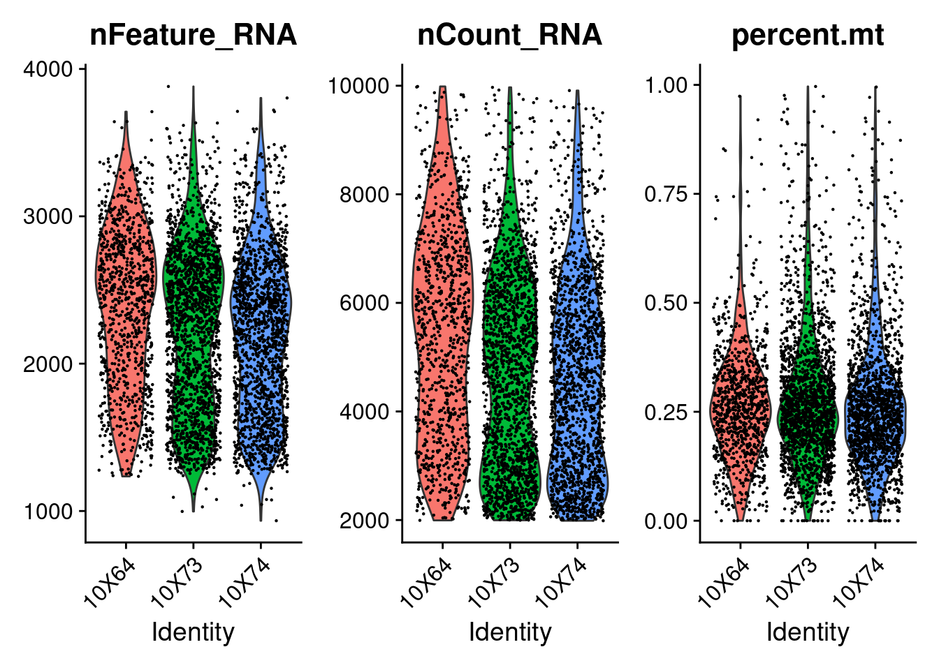
<- CreateSeuratObject (counts = getRawData (fb150Obj), project = "fb15.0" , min.cells = 3 , min.features = 200 )"percent.mt" ]] <- PercentageFeatureSet (seurat.obj, pattern = "^mt." )VlnPlot (seurat.obj, features = c ("nFeature_RNA" , "nCount_RNA" , "percent.mt" ), ncol = 3 )
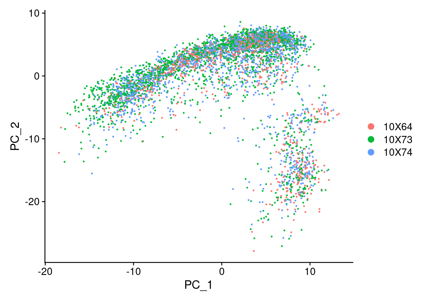
<- NormalizeData (seurat.obj, normalization.method = "LogNormalize" , scale.factor = 10000 )<- FindVariableFeatures (seurat.obj, selection.method = "vst" , nfeatures = 2000 )<- rownames (seurat.obj)<- ScaleData (seurat.obj, features = all.genes)<- RunPCA (seurat.obj, features = VariableFeatures (object = seurat.obj))DimPlot (seurat.obj)
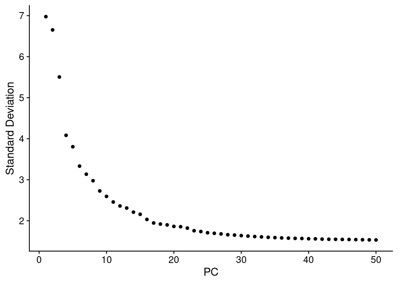
ElbowPlot (seurat.obj,ndims = 50 )
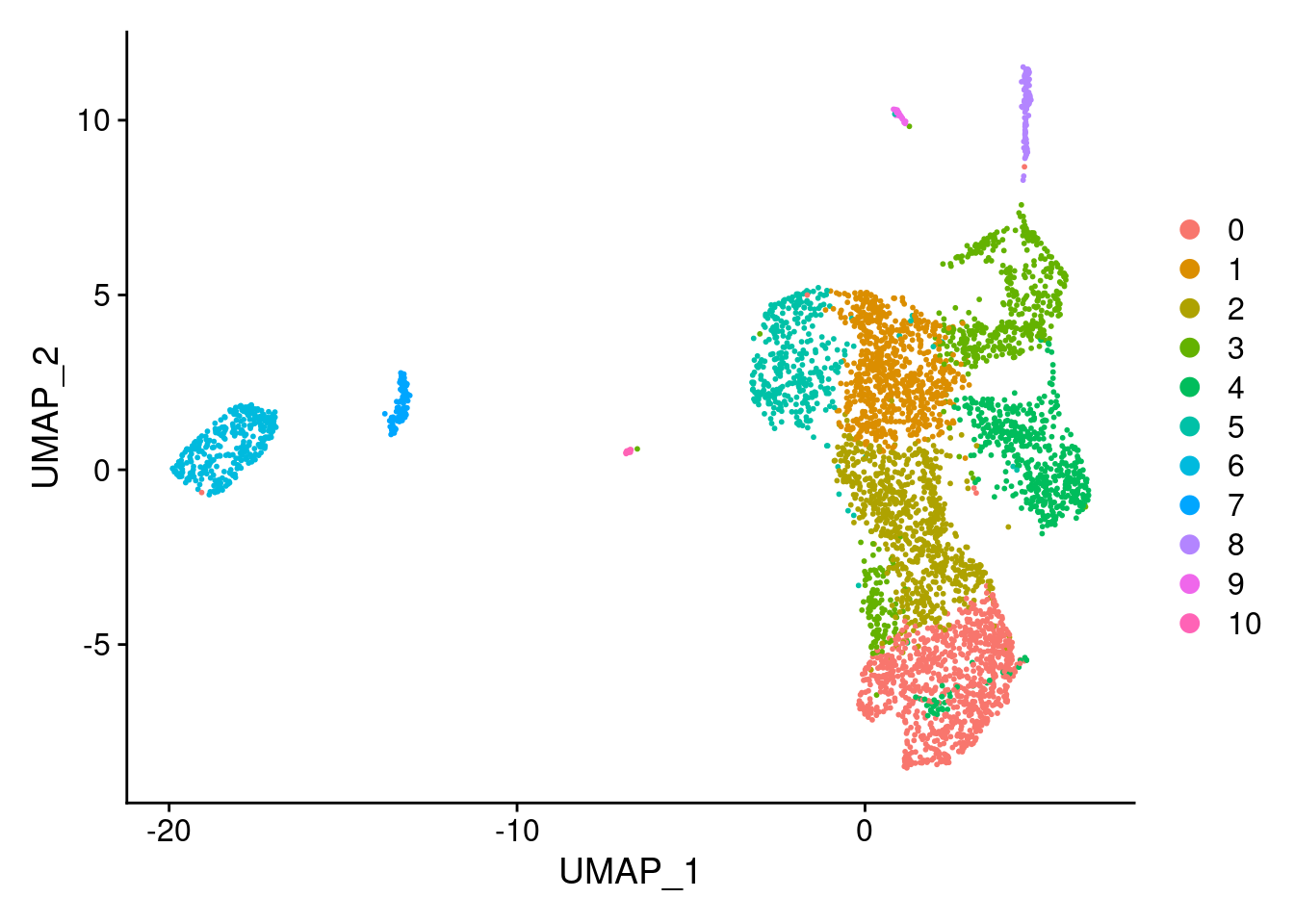
<- FindNeighbors (seurat.obj, dims = 1 : 25 )<- FindClusters (seurat.obj, resolution = 0.5 )
Modularity Optimizer version 1.3.0 by Ludo Waltman and Nees Jan van Eck

Number of nodes: 4407
Number of edges: 148076

Running Louvain algorithm...
Maximum modularity in 10 random starts: 0.8695
Number of communities: 11
Elapsed time: 0 seconds
<- RunUMAP (seurat.obj, dims = 1 : 25 )
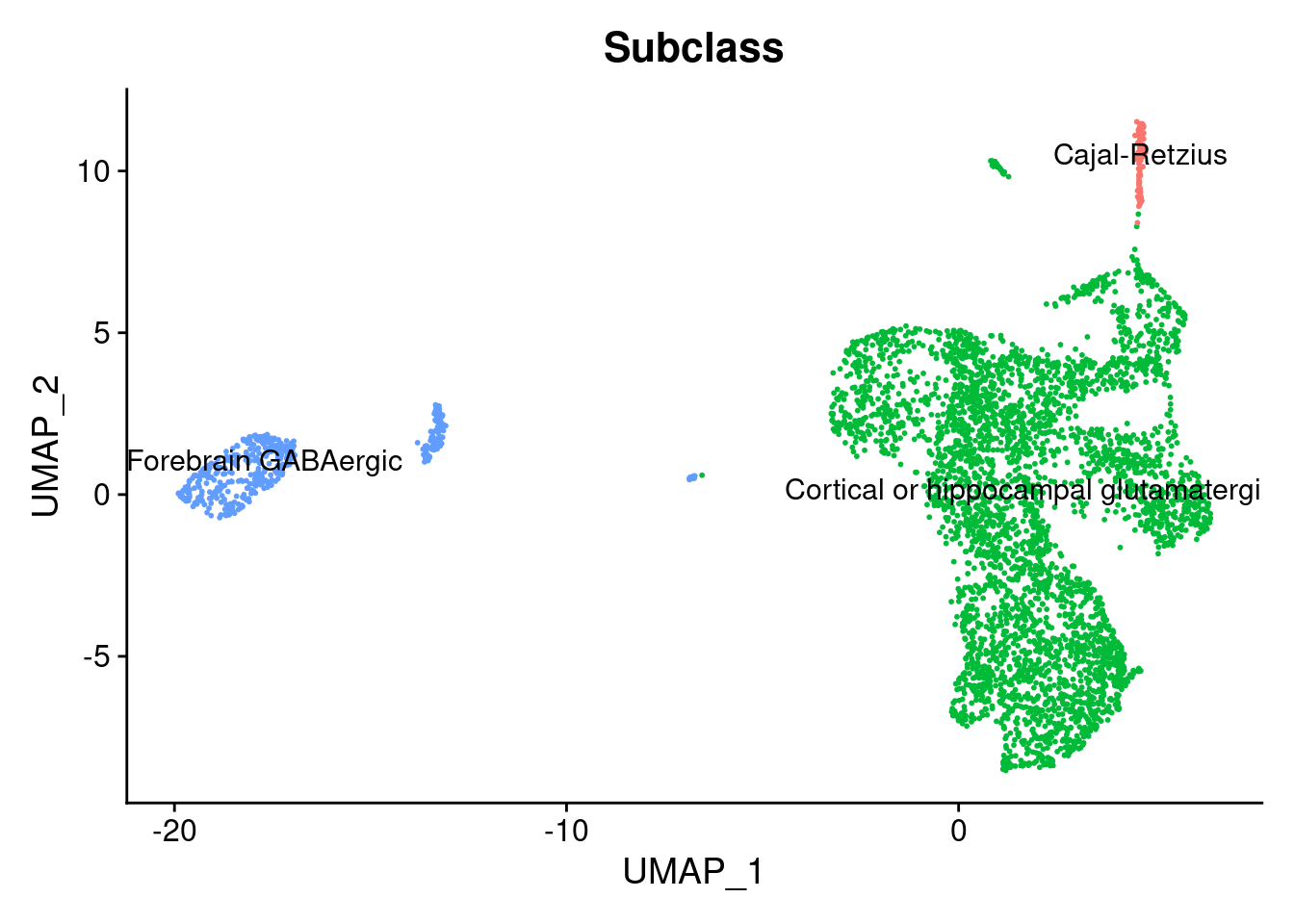
identical (rownames (seurat.obj@ meta.data),rownames (metaC))@ meta.data <- cbind (seurat.obj@ meta.data, metaC)DimPlot (seurat.obj,group.by = "Subclass" , label = TRUE )+ NoLegend ()
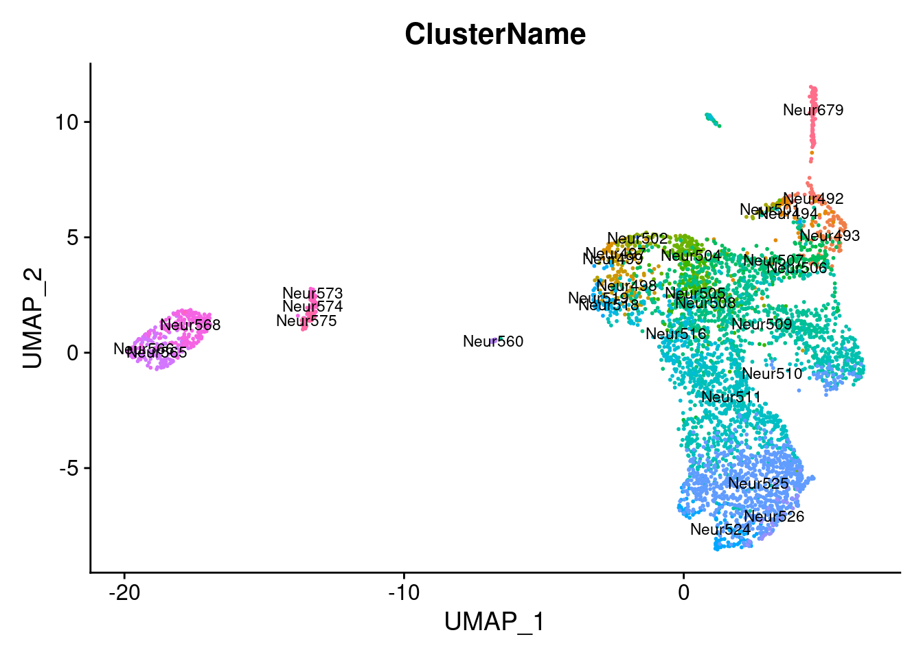
DimPlot (seurat.obj,group.by = "ClusterName" , label = T, label.size = 3 )+ NoLegend ()
<- SetIdent (seurat.obj,value = "Subclass" )<- FindAllMarkers (seurat.obj, logfc.threshold = 0.1 ,min.pct = 0.01 , only.pos = TRUE )head (seurat.obj.markers.Subclass)
                p_val avg_log2FC pct.1 pct.2     p_val_adj
Neurod6  0.000000e+00   4.090494 0.987 0.127  0.000000e+00
Neurod2 3.164351e-294   3.376326 0.957 0.065 4.101949e-290
Tiam2   4.807385e-256   3.542872 0.900 0.068 6.231813e-252
Sox5    2.989319e-249   3.598904 0.912 0.127 3.875055e-245
Ppp2r2b 9.140509e-235   2.193826 0.970 0.361 1.184884e-230
Rbfox1  3.234905e-206   2.318090 0.974 0.412 4.193407e-202
                                      cluster    gene
Neurod6 Cortical or hippocampal glutamatergic Neurod6
Neurod2 Cortical or hippocampal glutamatergic Neurod2
Tiam2   Cortical or hippocampal glutamatergic   Tiam2
Sox5    Cortical or hippocampal glutamatergic    Sox5
Ppp2r2b Cortical or hippocampal glutamatergic Ppp2r2b
Rbfox1  Cortical or hippocampal glutamatergic  Rbfox1
<- SetIdent (seurat.obj,value = "ClusterName" )<- FindAllMarkers (seurat.obj,densify = TRUE , logfc.threshold = 0.1 ,min.pct = 0.01 ,only.pos = TRUE )head (seurat.obj.markers.ClusterName)
                 p_val avg_log2FC pct.1 pct.2     p_val_adj cluster     gene
Wnt10a   4.836119e-259  0.9646853 0.316 0.000 6.269061e-255 Neur492   Wnt10a
Adamts19 2.737699e-201  0.8726592 0.316 0.001 3.548879e-197 Neur492 Adamts19
Tac2     1.894266e-172  2.0721515 0.316 0.002 2.455537e-168 Neur492     Tac2
Rmst     1.166934e-155  2.2966143 0.763 0.024 1.512697e-151 Neur492     Rmst
Eomes    1.978338e-139  1.6902540 0.579 0.015 2.564520e-135 Neur492    Eomes
Ebf1     4.915113e-109  1.9468755 0.526 0.016 6.371461e-105 Neur492     Ebf1
Comparision COTAN-Seurat
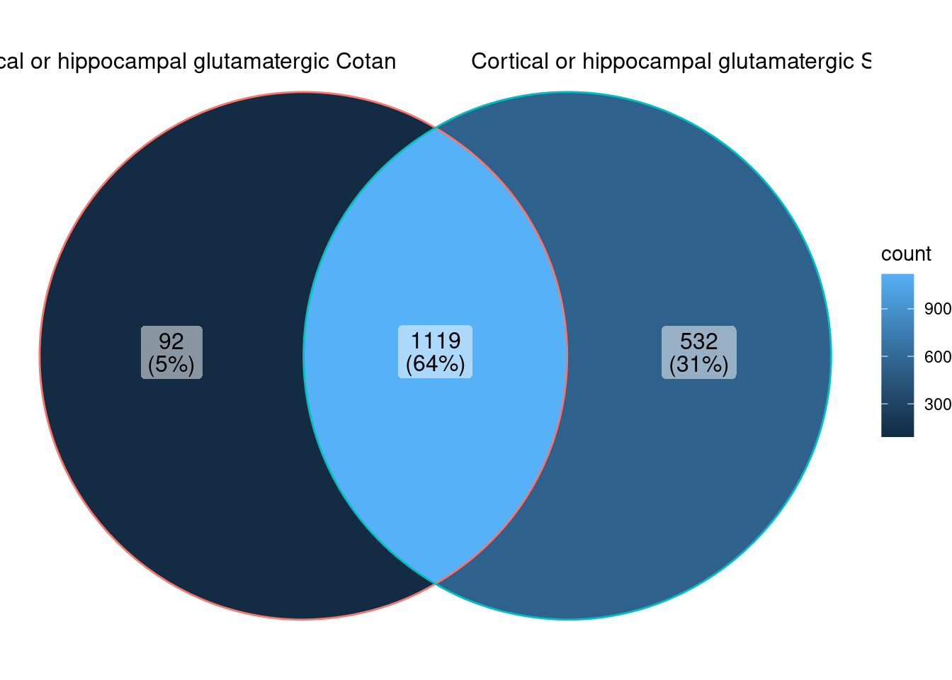
<- col_concat (crossing (colnames (dea.Subclass$ coex),c ("Seurat" ,"Cotan" )),sep = " " )<- vector ("list" , length (markers.list.names))names (markers.list) <- markers.list.names# I take positive coex significant genes for (cl.name in colnames (dea.Subclass$ coex)) {<- rownames (dea.Subclass$ coex[dea.Subclass$ ` p-value ` [,cl.name] < 0.01 & dea.Subclass$ coex[,cl.name] > 0 ,])paste0 (cl.name," Cotan" )]] <- genes#For seurat for (cl.name in colnames (dea.Subclass$ coex)) {<- seurat.obj.markers.Subclass[seurat.obj.markers.Subclass$ cluster == cl.name & seurat.obj.markers.Subclass$ p_val < 0.01 ,]$ genepaste0 (cl.name," Seurat" )]] <- genes
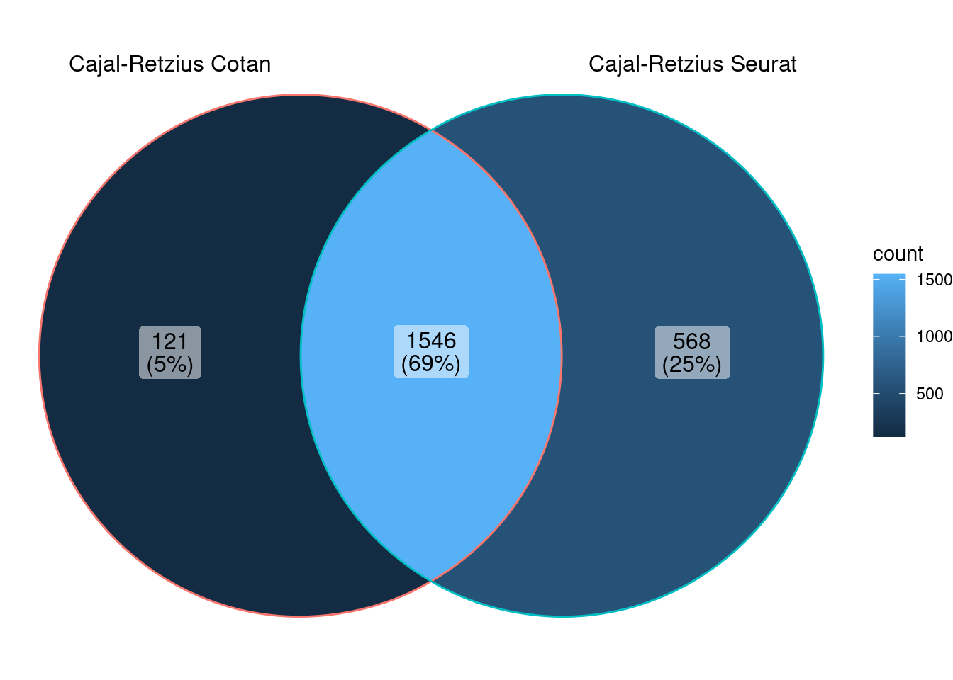
Cajal-Retzius subclass
<- ggVennDiagram (markers.list[1 : 2 ])
We can observe that there is a good overlap among the detected markers.
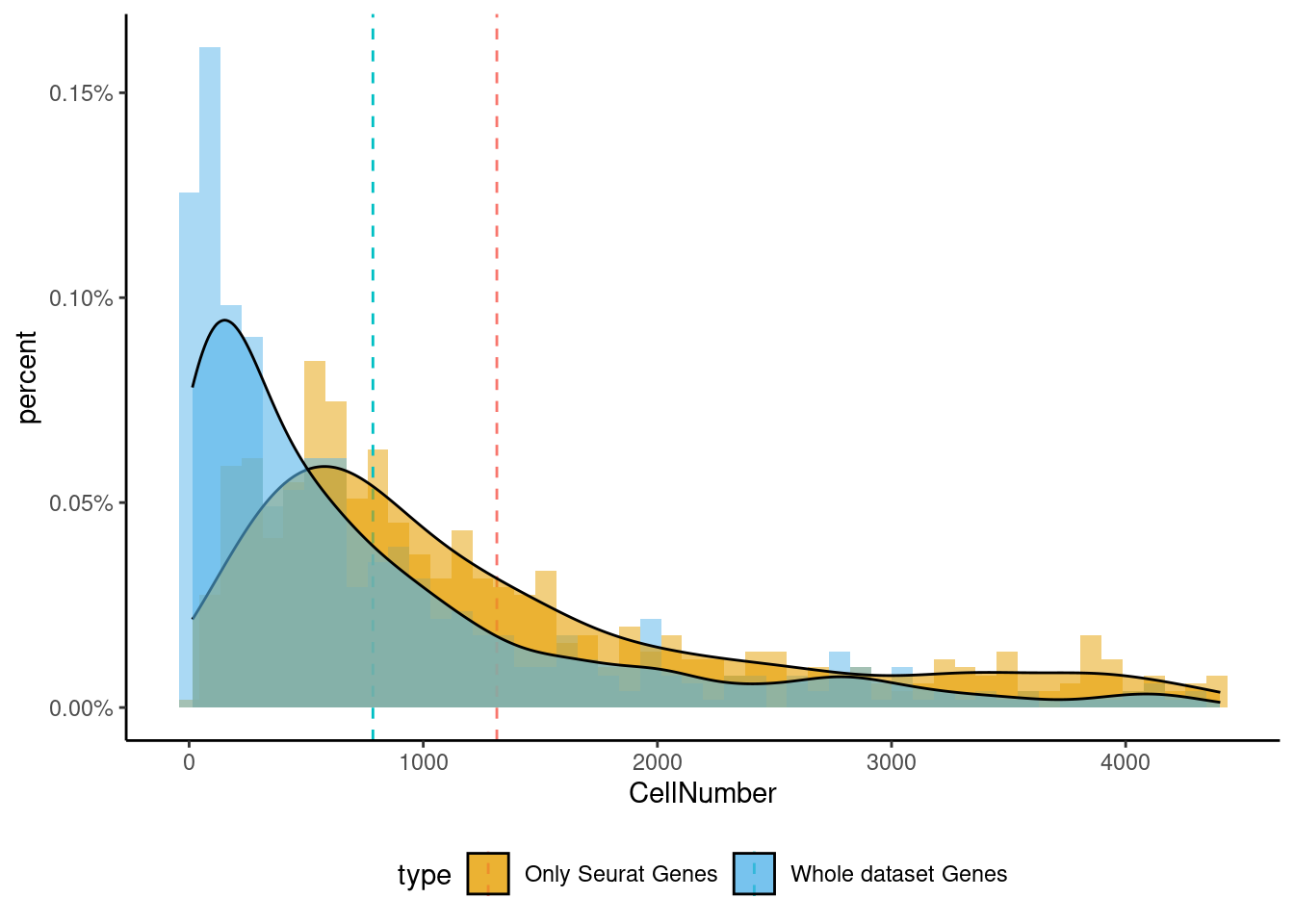
<- markers.list$ ` Cajal-Retzius Seurat ` [! markers.list$ ` Cajal-Retzius Seurat ` %in% markers.list$ ` Cajal-Retzius Cotan ` ]<- getNumOfExpressingCells (fb150Obj)[genes.to.test]<- as.data.frame (df)colnames (df) <- "CellNumber" rownames (df) <- NULL $ type <- "Only Seurat Genes" <- as.data.frame (getNumOfExpressingCells (fb150Obj)[sample (getGenes (fb150Obj), size = length (rownames (df)))])rownames (df.bk) <- NULL colnames (df.bk) <- "CellNumber" $ type <- "Whole dataset Genes" <- rbind (df,df.bk)<- ddply (df, "type" , summarise, grp.mean= mean (CellNumber))ggplot (df,aes (x= CellNumber,fill= type))+ scale_fill_manual (values= c ("#E69F00" , "#56B4E9" ))+ geom_histogram (aes (y= ..density..), position= "identity" , alpha= 0.5 ,bins = 50 )+ geom_vline (data= mu, aes (xintercept= grp.mean, color= type),linetype= "dashed" )+ geom_density (alpha= 0.6 )+ scale_y_continuous (labels = percent, name = "percent" ) + theme_classic ()+ theme (legend.position= "bottom" )
set.seed (111 )<- sample (genes.to.test,size = 12 )
 [1] "Zfp579" "Lias"   "Tmed2"  "Srsf9"  "Dtx3"   "Srp14"  "Pofut2" "Rtn1"
 [9] "Thap3"  "Cttn"   "Socs2"  "Ctxn1"
= 0 for (g in c (0 : 2 )) {= g* 4 plot (FeaturePlot (seurat.obj,features = genes[n+ c (1 : 4 )], label = T))
Generally if we look at the genes specifically detected by Seurat, they don’t seems so distinctive for CR cells.
sum (genes.to.test %in% markers.list$ ` Cortical or hippocampal glutamatergic Seurat ` )/ length (genes.to.test)
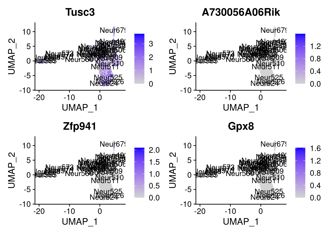
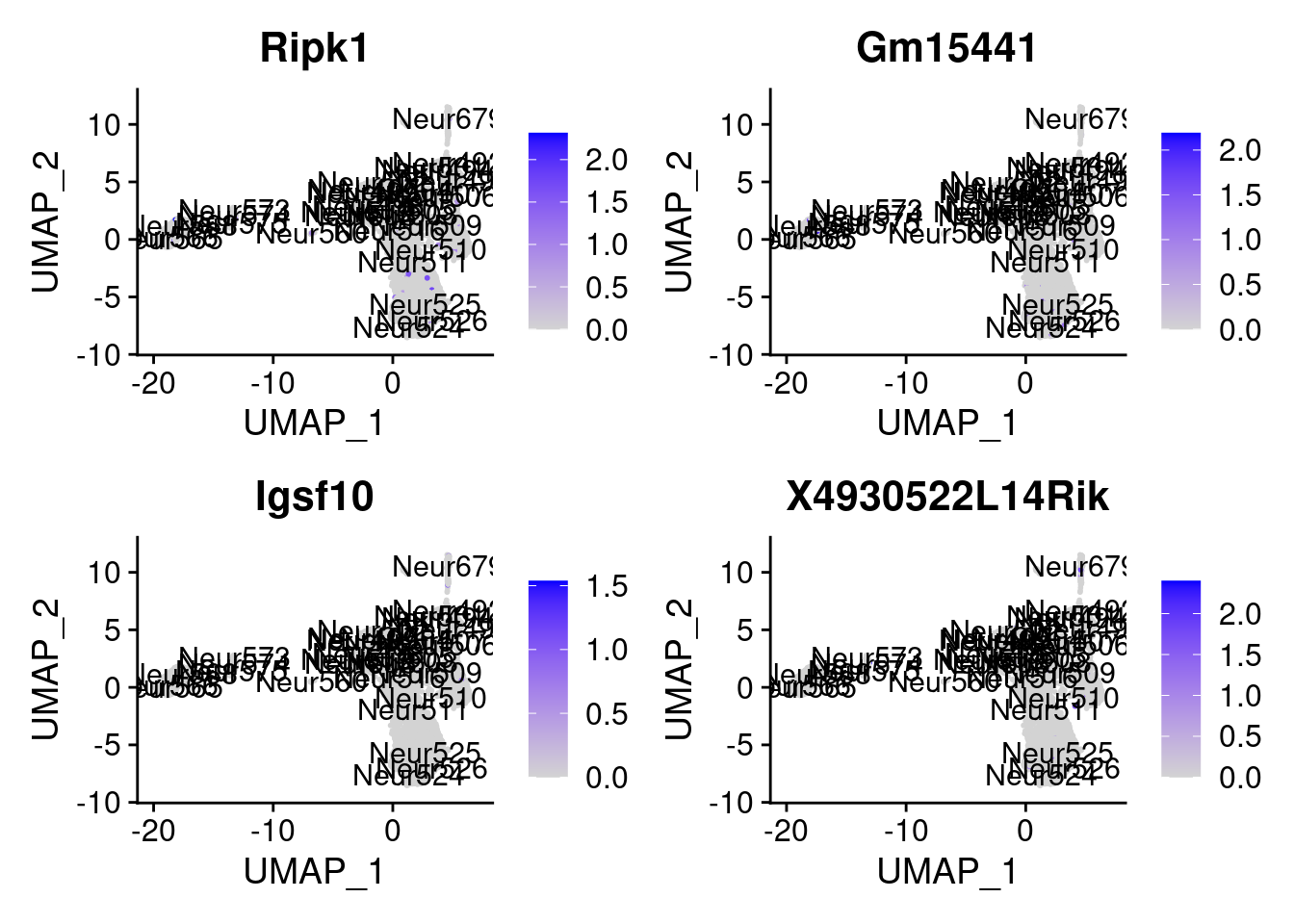
<- markers.list$ ` Cajal-Retzius Cotan ` [! markers.list$ ` Cajal-Retzius Cotan ` %in% markers.list$ ` Cajal-Retzius Seurat ` ]set.seed (11 )<- sample (genes.to.test.Cotan,size = 30 )
 [1] "Fam149a"        "Slc35g2"        "Chst7"          "P2ry14"
 [5] "Tusc3"          "A730056A06Rik"  "Zfp941"         "Gpx8"
 [9] "Ripk1"          "Gm15441"        "Igsf10"         "X4930522L14Rik"
[13] "Gm16845"        "Gspt2"          "Scn2b"          "Akr1b10"
[17] "Vegfa"          "X4933431E20Rik" "Rtkn"           "Gm38250"
[21] "Fancf"          "Rab43"          "Grik1"          "Eya1"
[25] "Pih1d2"         "Cldn12"         "Cacng2"         "Pias3"
[29] "Gm26782"        "Mme"
= 0 for (g in c (0 : 2 )) {= g* 4 plot (FeaturePlot (seurat.obj,features = genes[n+ c (1 : 4 )], label = T))
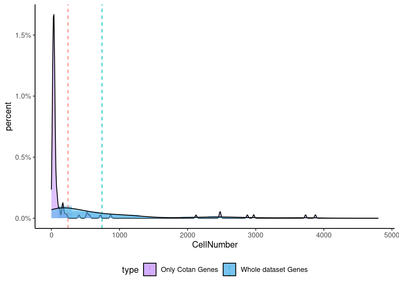
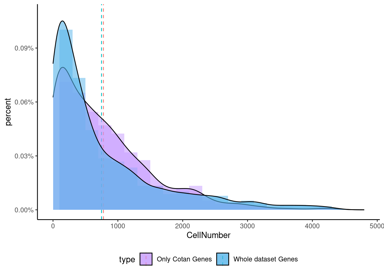
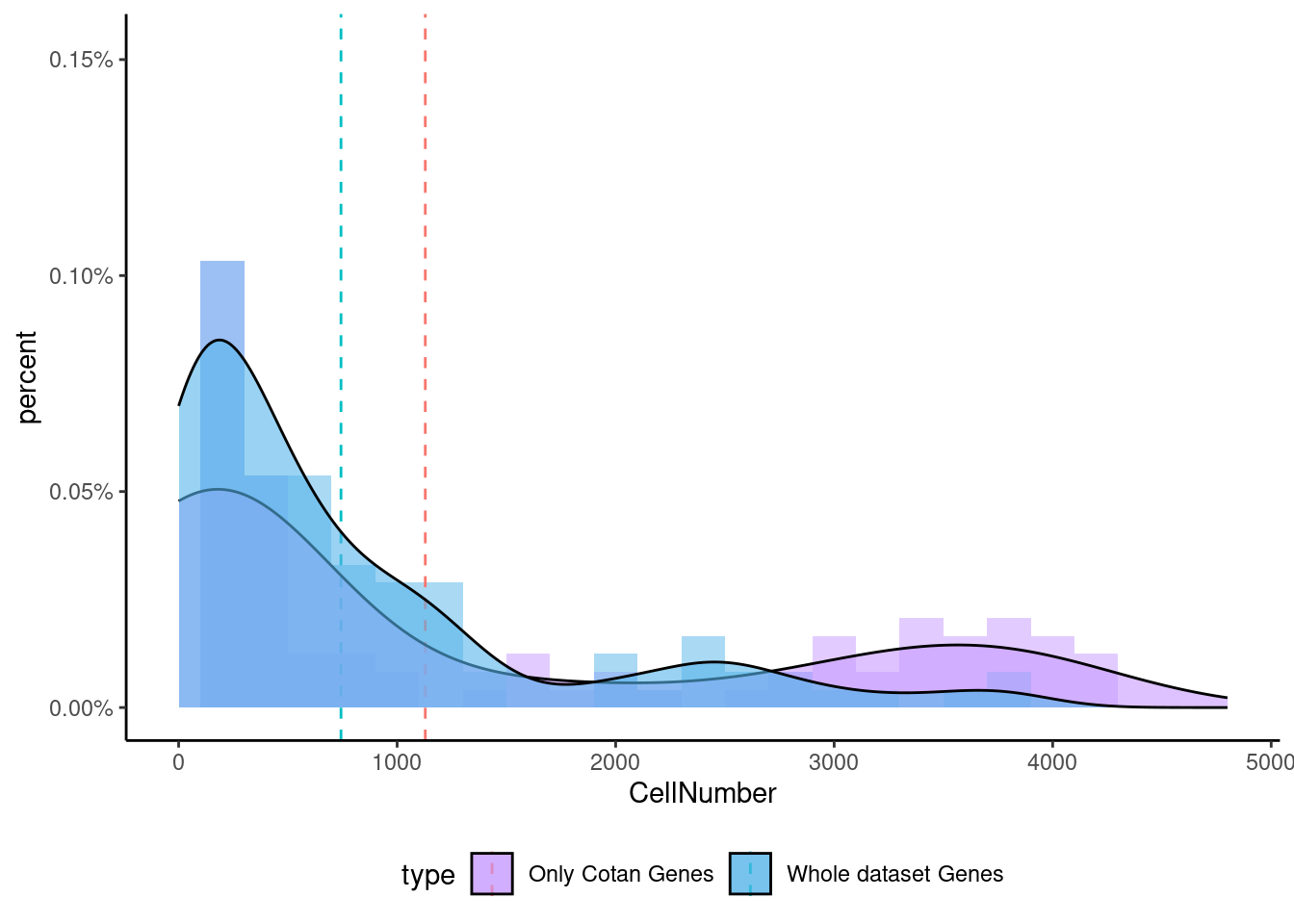
<- getNumOfExpressingCells (fb150Obj)[genes.to.test.Cotan]<- as.data.frame (df)colnames (df) <- "CellNumber" rownames (df) <- NULL $ type <- "Only Cotan Genes" <- as.data.frame (getNumOfExpressingCells (fb150Obj)[sample (getGenes (fb150Obj), size = length (rownames (df)))])rownames (df.bk) <- NULL colnames (df.bk) <- "CellNumber" $ type <- "Whole dataset Genes" <- rbind (df,df.bk)<- ddply (df, "type" , summarise, grp.mean= mean (CellNumber))ggplot (df,aes (x= CellNumber,fill= type))+ scale_fill_manual (values= c ("#C69AFF" , "#56B4E9" ))+ geom_histogram (aes (y= ..density..), position= "identity" , alpha= 0.5 ,bins = 25 )+ xlim (0 ,4800 )+ geom_vline (data= mu, aes (xintercept= grp.mean, color= type),linetype= "dashed" )+ geom_density (alpha= 0.6 )+ scale_y_continuous (labels = percent, name = "percent" ) + theme_classic ()+ theme (legend.position= "bottom" )
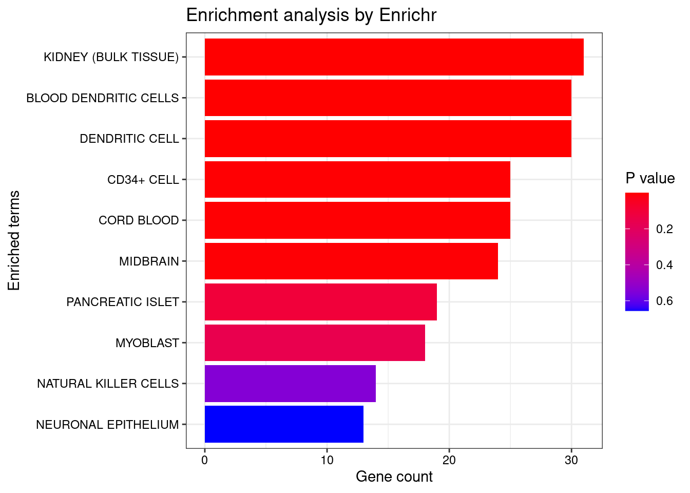
Now we can test the enrichment for the specific gene both in Seurat and in Cotan.
To make a comparison more equal we select the same number of genes (depending on the smallest group)
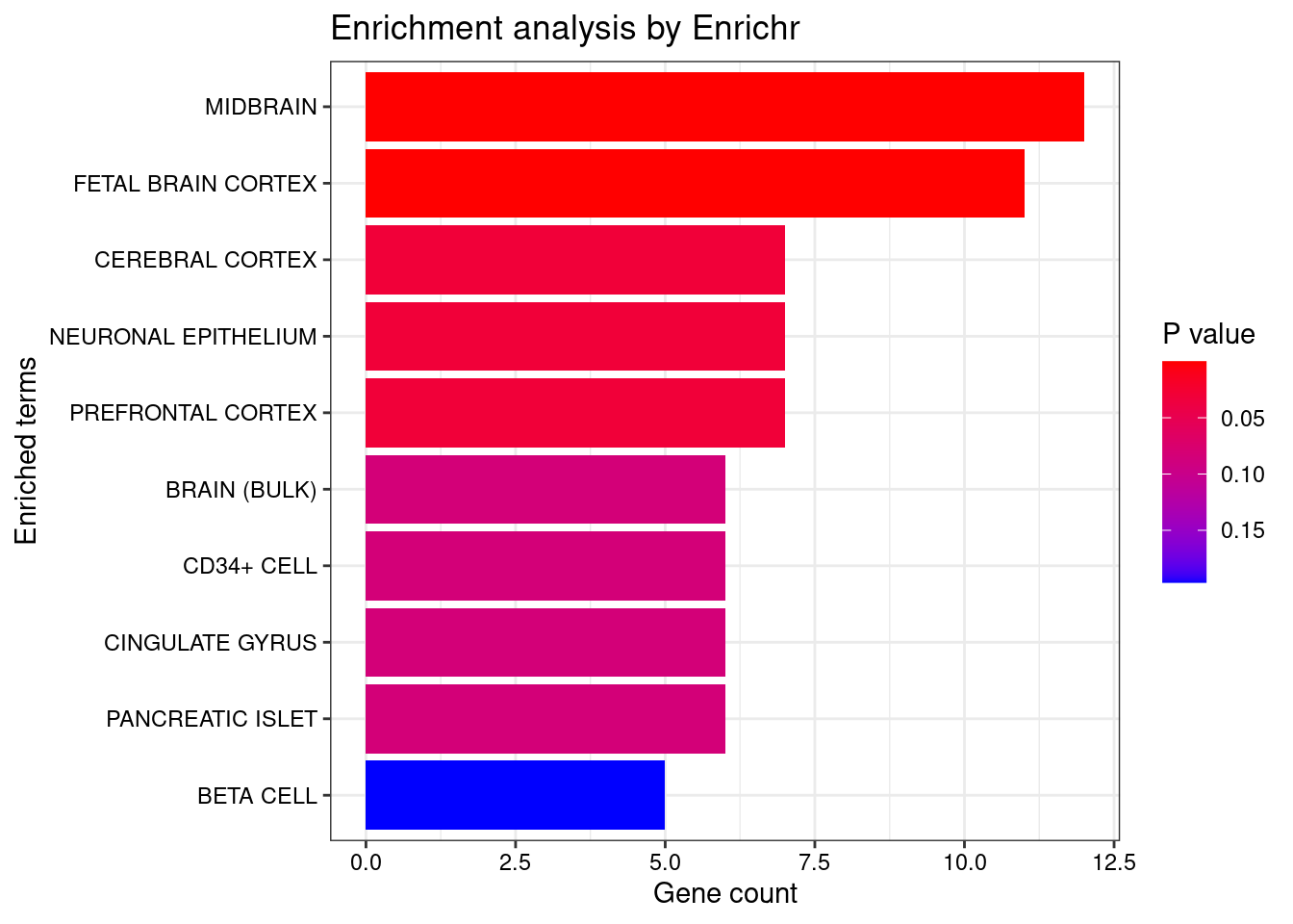
<- seurat.obj.markers.Subclass[seurat.obj.markers.Subclass$ cluster == "Cajal-Retzius" & seurat.obj.markers.Subclass$ gene %in% genes.to.test,]$ gene[1 : length (genes.to.test.Cotan)]<- enrichr (genes.to.testTop, dbs)
Uploading data to Enrichr... Done.
  Querying ARCHS4_Tissues... Done.
Parsing results... Done.
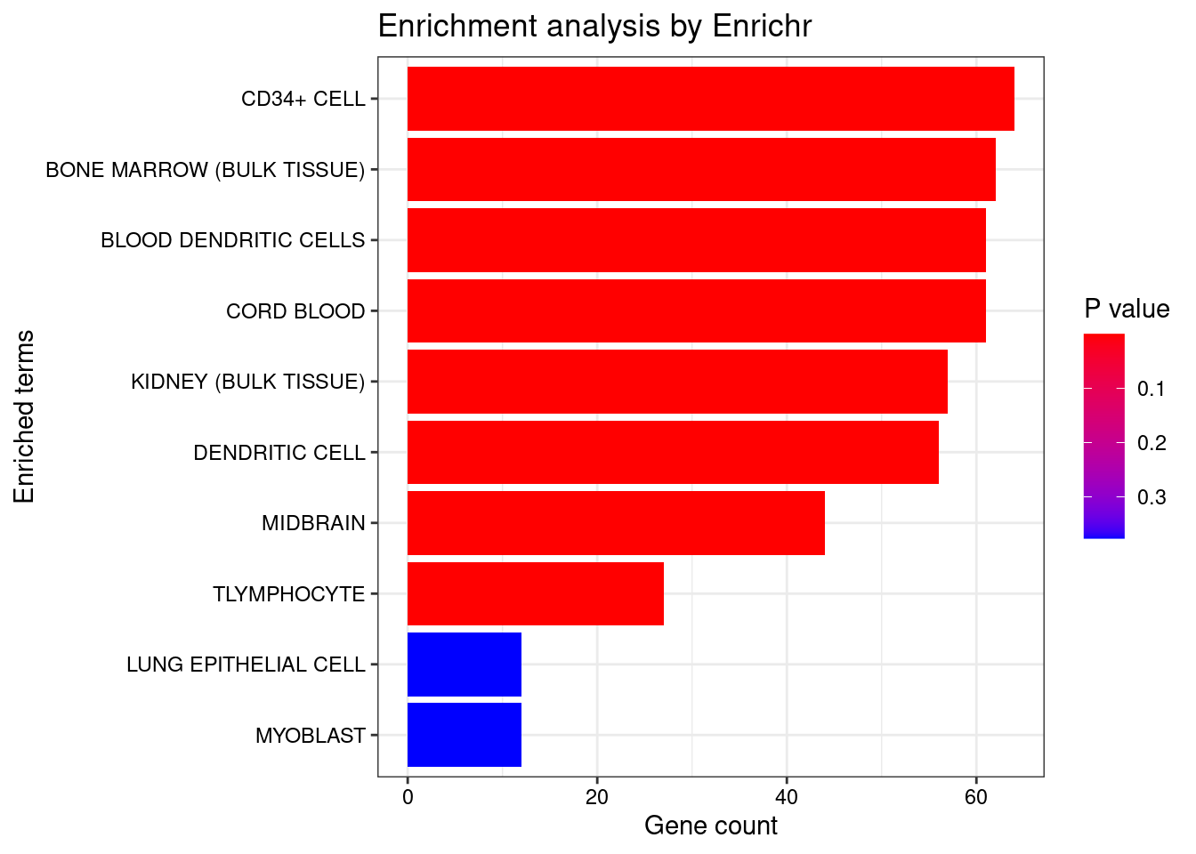
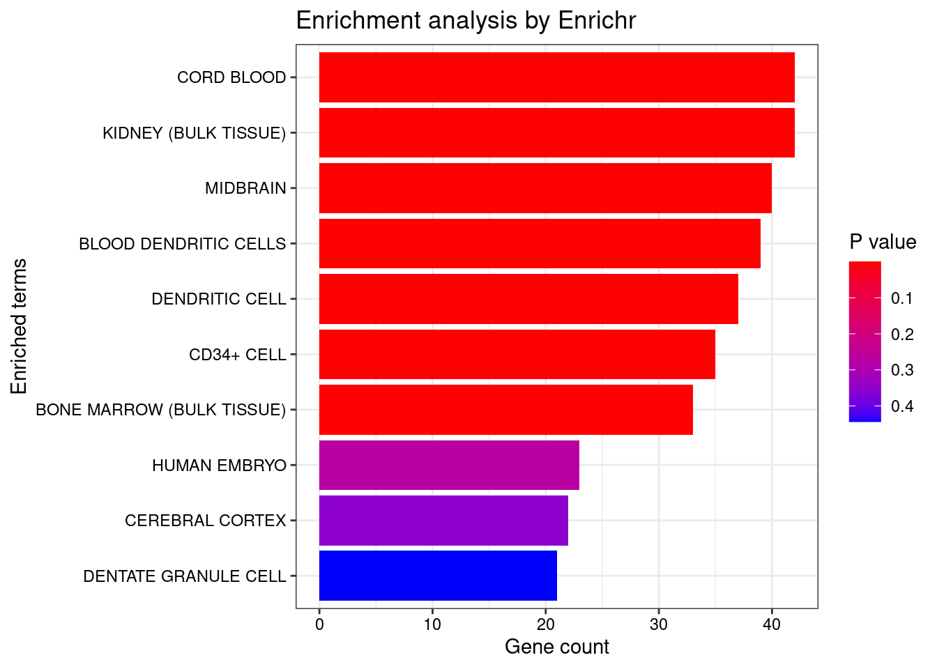
plotEnrich (enriched[[1 ]], showTerms = 10 , numChar = 40 , y = "Count" , orderBy = "P.value" )
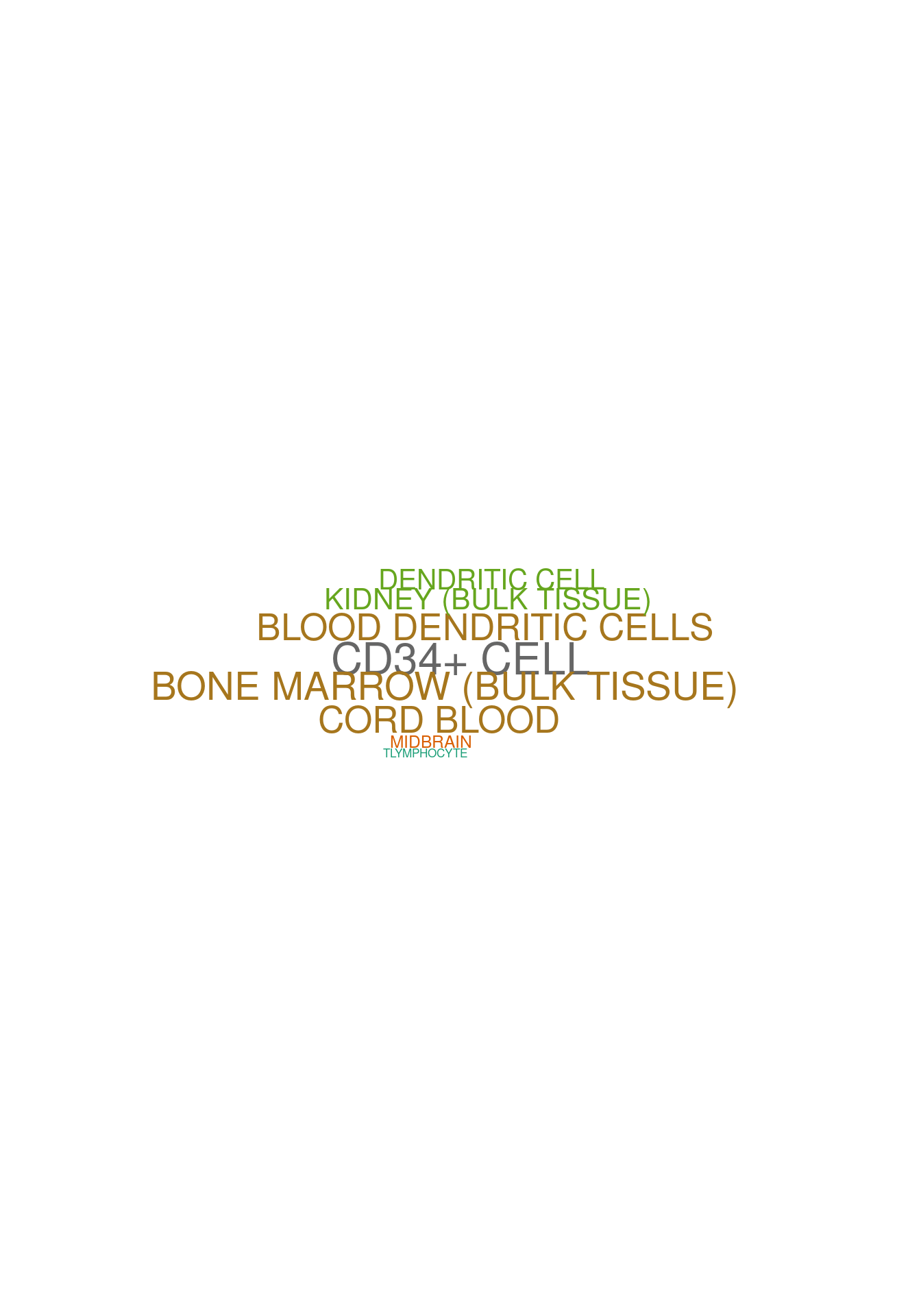
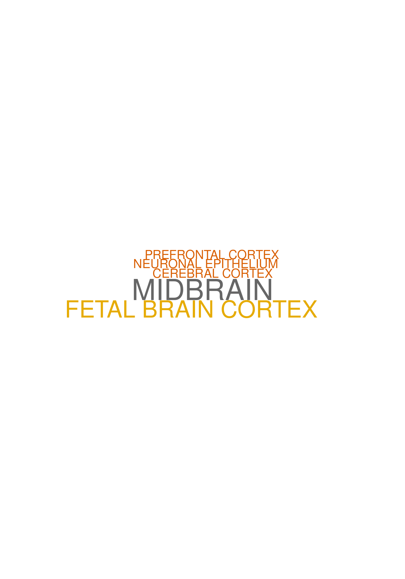
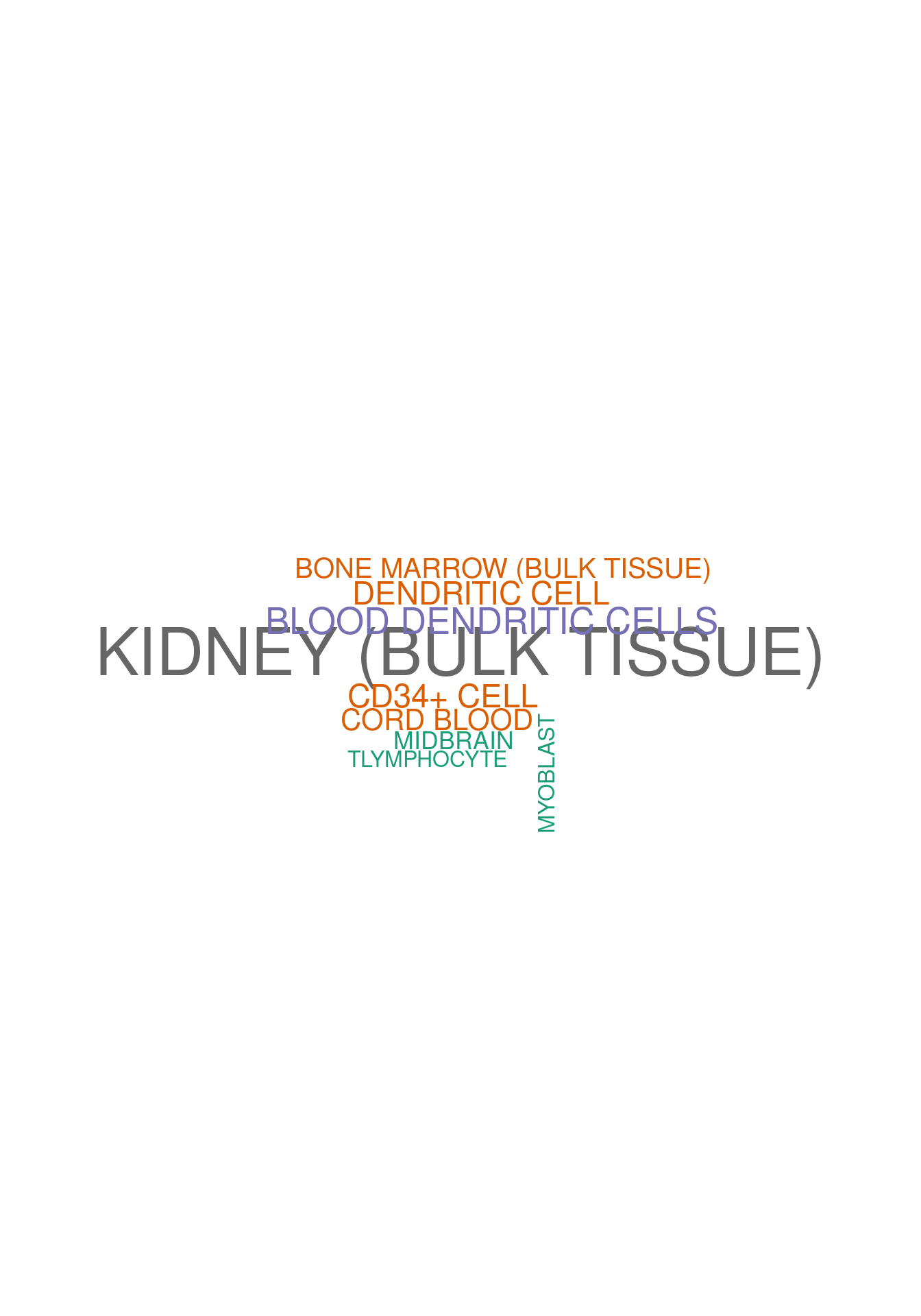
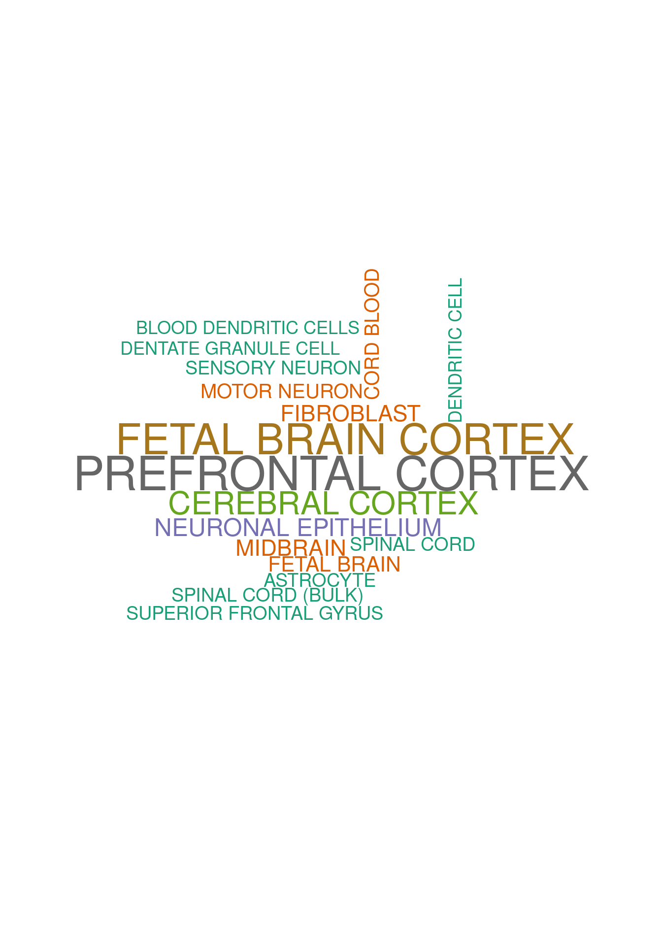
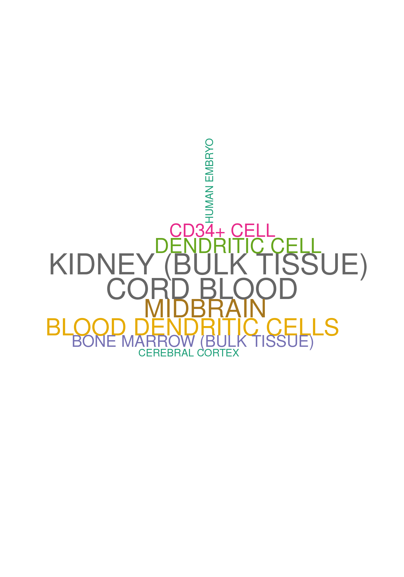
set.seed (123 )<- data.frame (Terms = str_split (enriched[[1 ]]$ Term[1 : 20 ],pattern = " CL" ,simplify = T )[,1 ],Scores = enriched[[1 ]]$ Combined.Score[1 : 20 ])wordcloud (wordcloud_data$ Terms, wordcloud_data$ Scores, scale = c (3 , 1 ), min.freq = 1 , random.order= FALSE , rot.per= 0.1 ,colors= brewer.pal (8 , "Dark2" ))
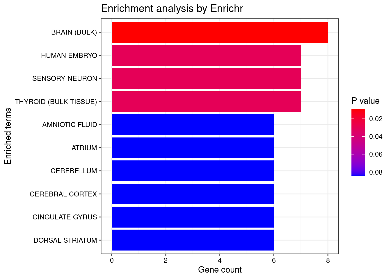
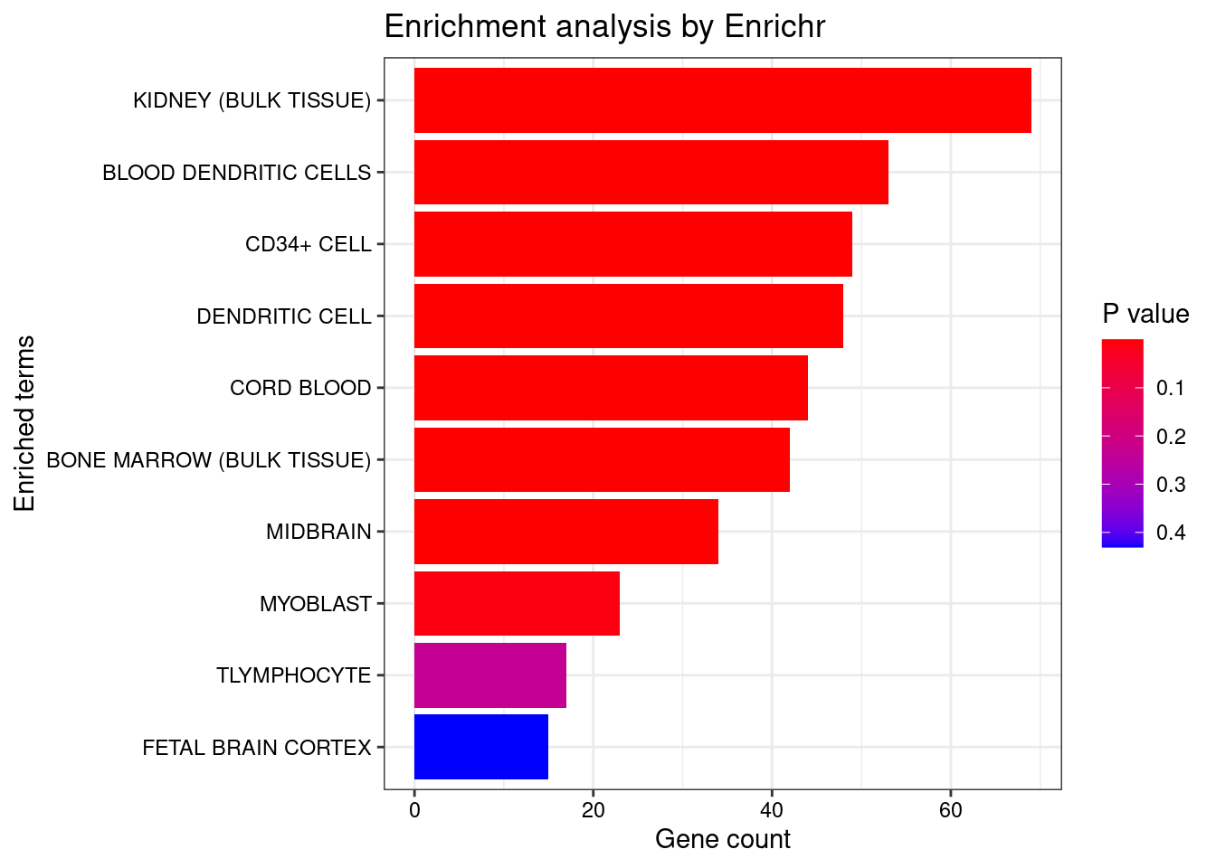
<- enrichr (genes.to.test.Cotan, dbs)
Uploading data to Enrichr... Done.
  Querying ARCHS4_Tissues... Done.
Parsing results... Done.
plotEnrich (enriched[[1 ]], showTerms = 10 , numChar = 40 , y = "Count" , orderBy = "P.value" )
set.seed (123 )<- data.frame (Terms = str_split (enriched[[1 ]]$ Term[1 : 20 ],pattern = " CL" ,simplify = T )[,1 ],Scores = enriched[[1 ]]$ Combined.Score[1 : 20 ])wordcloud (wordcloud_data$ Terms, wordcloud_data$ Scores, scale = c (3 , 1 ), min.freq = 1 , random.order= FALSE , rot.per= 0.1 ,colors= brewer.pal (8 , "Dark2" ))
Cortical or hippocampal glutamatergic subclass
<- ggVennDiagram (markers.list[3 : 4 ])
<- markers.list$ ` Cortical or hippocampal glutamatergic Seurat ` [! markers.list$ ` Cortical or hippocampal glutamatergic Seurat ` %in% markers.list$ ` Cortical or hippocampal glutamatergic Cotan ` ]<- getNumOfExpressingCells (fb150Obj)[genes.to.test]<- as.data.frame (df)colnames (df) <- "CellNumber" rownames (df) <- NULL $ type <- "Only Seurat Genes" <- as.data.frame (getNumOfExpressingCells (fb150Obj)[sample (getGenes (fb150Obj), size = length (rownames (df)))])rownames (df.bk) <- NULL colnames (df.bk) <- "CellNumber" $ type <- "Whole dataset Genes" <- rbind (df,df.bk)library (plyr)library (scales) <- ddply (df, "type" , summarise, grp.mean= mean (CellNumber))ggplot (df,aes (x= CellNumber,fill= type))+ scale_fill_manual (values= c ("#E69F00" , "#56B4E9" ))+ geom_histogram (aes (y= ..density..), position= "identity" , alpha= 0.5 ,bins = 50 )+ geom_vline (data= mu, aes (xintercept= grp.mean, color= type),linetype= "dashed" )+ geom_density (alpha= 0.6 )+ scale_y_continuous (labels = percent, name = "percent" ) + theme_classic ()+ theme (legend.position= "bottom" )
set.seed (111 )<- sample (genes.to.test,size = 18 )
 [1] "Fam220a" "Taok3"   "Fau"     "Fzd1"    "Rpl7"    "Idh3a"   "Lgmn"
 [8] "Mapkap1" "Apopt1"  "Tubg1"   "Rpl10"   "Rpl6"    "Ankrd45" "Nsa2"
[15] "Reep2"   "Rpl14"   "Egfem1"  "Letm1"
= 0 for (g in c (0 : 2 )) {= g* 4 plot (FeaturePlot (seurat.obj,features = genes[n+ c (1 : 4 )], label = T))
<- markers.list$ ` Cortical or hippocampal glutamatergic Cotan ` [! markers.list$ ` Cortical or hippocampal glutamatergic Cotan ` %in% markers.list$ ` Cortical or hippocampal glutamatergic Seurat ` ]set.seed (11 )<- sample (genes.to.test.Cotan,size = 30 )
 [1] "Pitpnm1"        "Nptx1"          "Tnfaip8l1"      "Dlc1"
 [5] "Ttyh1"          "Pde11a"         "Adamts2"        "Pomk"
 [9] "D6Ertd474e"     "Car12"          "Rspo3"          "Gm43517"
[13] "X3830406C13Rik" "Grp"            "E2f1"           "Ntf3"
[17] "Stim2"          "D030068K23Rik"  "Tspan17"        "Ube2t"
[21] "Impa2"          "Egfl6"          "Serping1"       "Pttg1"
[25] "Sh3bgrl3"       "Mcrip2"         "Map1lc3a"       "Nrn1"
[29] "Gm42997"        "AC124490.1"
= 0 for (g in c (0 : 2 )) {= g* 4 plot (FeaturePlot (seurat.obj,features = genes[n+ c (1 : 4 )], label = T))
<- getNumOfExpressingCells (fb150Obj)[genes.to.test.Cotan]<- as.data.frame (df)colnames (df) <- "CellNumber" rownames (df) <- NULL $ type <- "Only Cotan Genes" <- as.data.frame (getNumOfExpressingCells (fb150Obj)[sample (getGenes (fb150Obj), size = length (rownames (df)))])rownames (df.bk) <- NULL colnames (df.bk) <- "CellNumber" $ type <- "Whole dataset Genes" <- rbind (df,df.bk)<- ddply (df, "type" , summarise, grp.mean= mean (CellNumber))ggplot (df,aes (x= CellNumber,fill= type))+ scale_fill_manual (values= c ("#C69AFF" , "#56B4E9" ))+ geom_histogram (aes (y= ..density..), position= "identity" , alpha= 0.5 ,bins = 25 )+ xlim (0 ,4800 )+ geom_vline (data= mu, aes (xintercept= grp.mean, color= type),linetype= "dashed" )+ geom_density (alpha= 0.6 )+ scale_y_continuous (labels = percent, name = "percent" ) + theme_classic ()+ theme (legend.position= "bottom" )
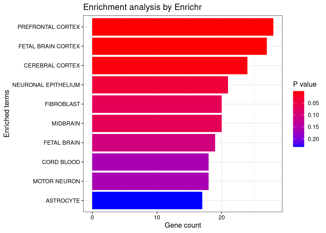
<- seurat.obj.markers.Subclass[seurat.obj.markers.Subclass$ cluster == "Cortical or hippocampal glutamatergic" & seurat.obj.markers.Subclass$ gene %in% genes.to.test,]$ gene[1 : length (genes.to.test.Cotan)]<- enrichr (genes.to.testTop, dbs)
Uploading data to Enrichr... Done.
  Querying ARCHS4_Tissues... Done.
Parsing results... Done.
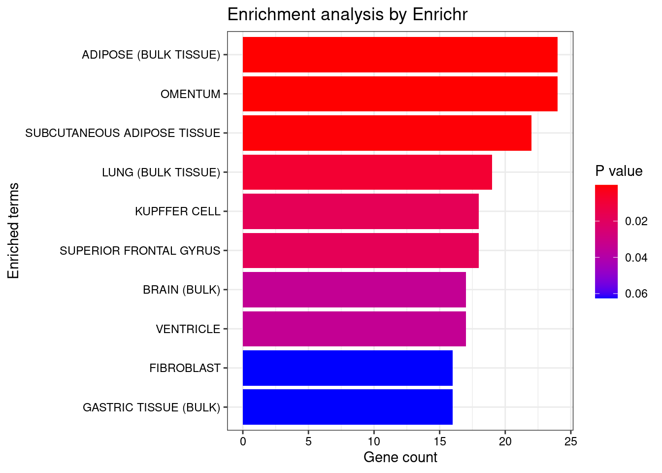
plotEnrich (enriched[[1 ]], showTerms = 10 , numChar = 40 , y = "Count" , orderBy = "P.value" )
set.seed (12333 )<- data.frame (Terms = str_split (enriched[[1 ]]$ Term[1 : 8 ],pattern = " CL" ,simplify = T )[,1 ],Scores = enriched[[1 ]]$ Combined.Score[1 : 8 ])wordcloud (wordcloud_data$ Terms, wordcloud_data$ Scores, scale = c (2 , 0.5 ), min.freq = 1 , random.order= FALSE , rot.per= 0.1 ,colors= brewer.pal (8 , "Dark2" ))
<- enrichr (genes.to.test.Cotan, dbs)
Uploading data to Enrichr... Done.
  Querying ARCHS4_Tissues... Done.
Parsing results... Done.
plotEnrich (enriched[[1 ]], showTerms = 10 , numChar = 40 , y = "Count" , orderBy = "P.value" )
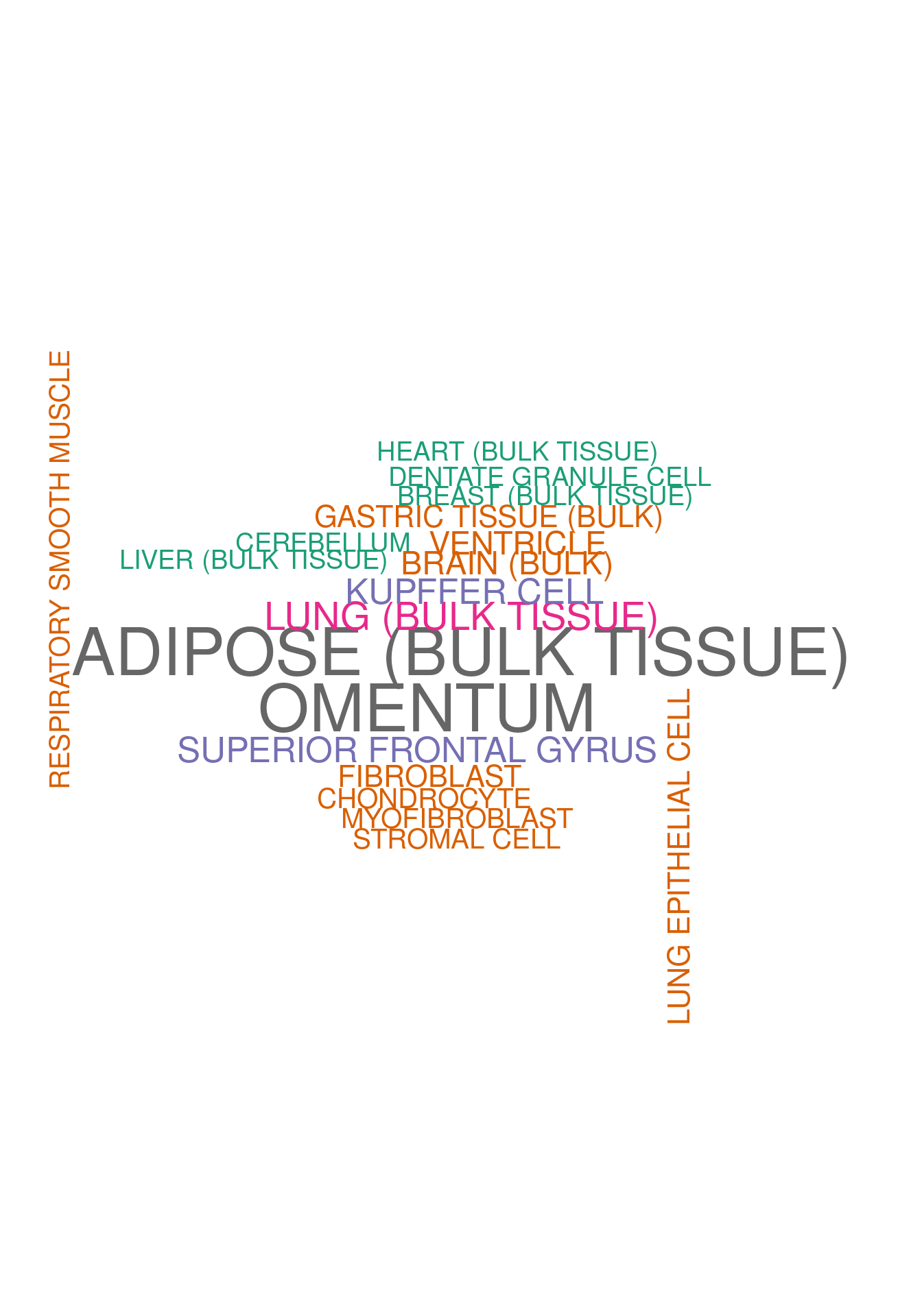
set.seed (1233 )<- data.frame (Terms = str_split (enriched[[1 ]]$ Term[1 : 20 ],pattern = " CL" ,simplify = T )[,1 ],Scores = enriched[[1 ]]$ Combined.Score[1 : 20 ])wordcloud (wordcloud_data$ Terms, wordcloud_data$ Scores, scale = c (3 , 1 ), min.freq = 1 , random.order= FALSE , rot.per= 0.1 ,colors= brewer.pal (8 , "Dark2" ))
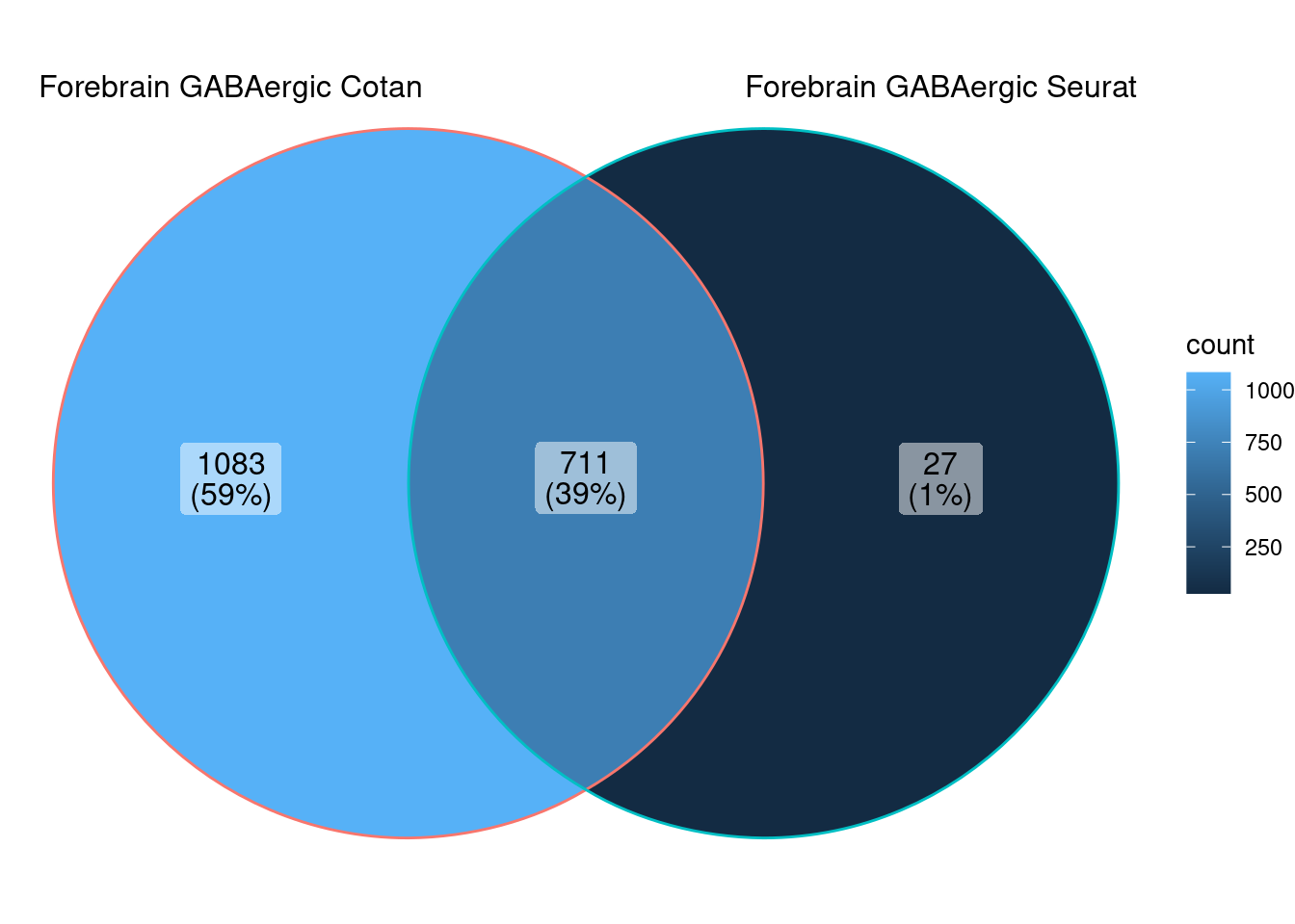
Forebrain GABAergic subclass
<- ggVennDiagram (markers.list[5 : 6 ])
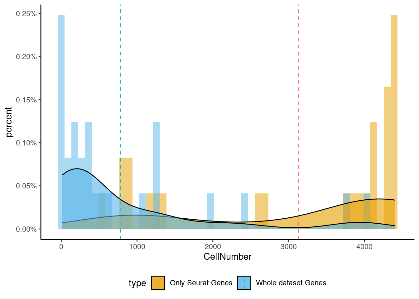
<- markers.list$ ` Forebrain GABAergic Seurat ` [! markers.list$ ` Forebrain GABAergic Seurat ` %in% markers.list$ ` Forebrain GABAergic Cotan ` ]<- getNumOfExpressingCells (fb150Obj)[genes.to.test]<- as.data.frame (df)colnames (df) <- "CellNumber" rownames (df) <- NULL $ type <- "Only Seurat Genes" <- as.data.frame (getNumOfExpressingCells (fb150Obj)[sample (getGenes (fb150Obj), size = length (rownames (df)))])rownames (df.bk) <- NULL colnames (df.bk) <- "CellNumber" $ type <- "Whole dataset Genes" <- rbind (df,df.bk)library (plyr)library (scales) <- ddply (df, "type" , summarise, grp.mean= mean (CellNumber))ggplot (df,aes (x= CellNumber,fill= type))+ scale_fill_manual (values= c ("#E69F00" , "#56B4E9" ))+ geom_histogram (aes (y= ..density..), position= "identity" , alpha= 0.5 ,bins = 50 )+ geom_vline (data= mu, aes (xintercept= grp.mean, color= type),linetype= "dashed" )+ geom_density (alpha= 0.6 )+ scale_y_continuous (labels = percent, name = "percent" ) + theme_classic ()+ theme (legend.position= "bottom" )
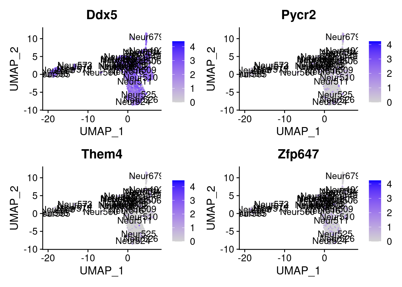
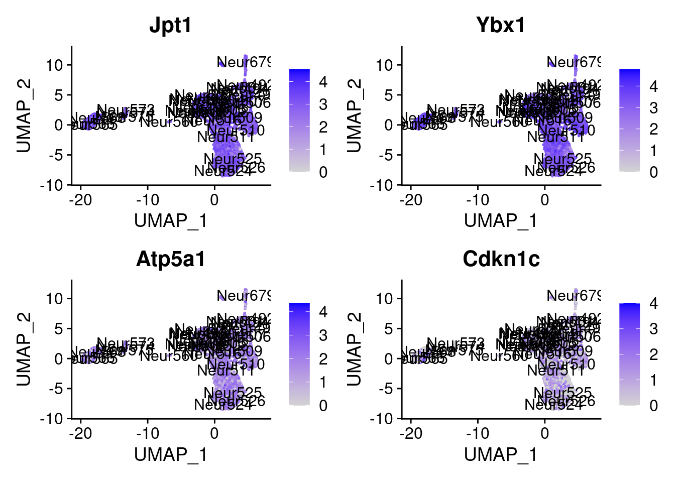
set.seed (111 )<- sample (genes.to.test,size = 18 )
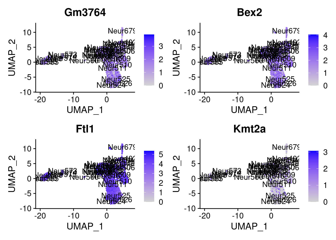
 [1] "Ddx5"    "Pycr2"   "Them4"   "Zfp647"  "Jpt1"    "Ybx1"    "Atp5a1"
 [8] "Cdkn1c"  "Gm3764"  "Bex2"    "Ftl1"    "Kmt2a"   "Map2"    "Cntnap2"
[15] "Pogk"    "Rtn1"    "Scg5"    "H3f3b"
= 0 for (g in c (0 : 2 )) {= g* 4 plot (FeaturePlot (seurat.obj,features = genes[n+ c (1 : 4 )], label = T))
<- markers.list$ ` Forebrain GABAergic Cotan ` [! markers.list$ ` Forebrain GABAergic Cotan ` %in% markers.list$ ` Forebrain GABAergic Seurat ` ]set.seed (11 )<- sample (genes.to.test.Cotan,size = 30 )
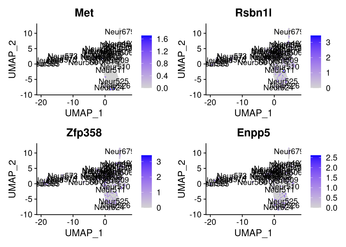
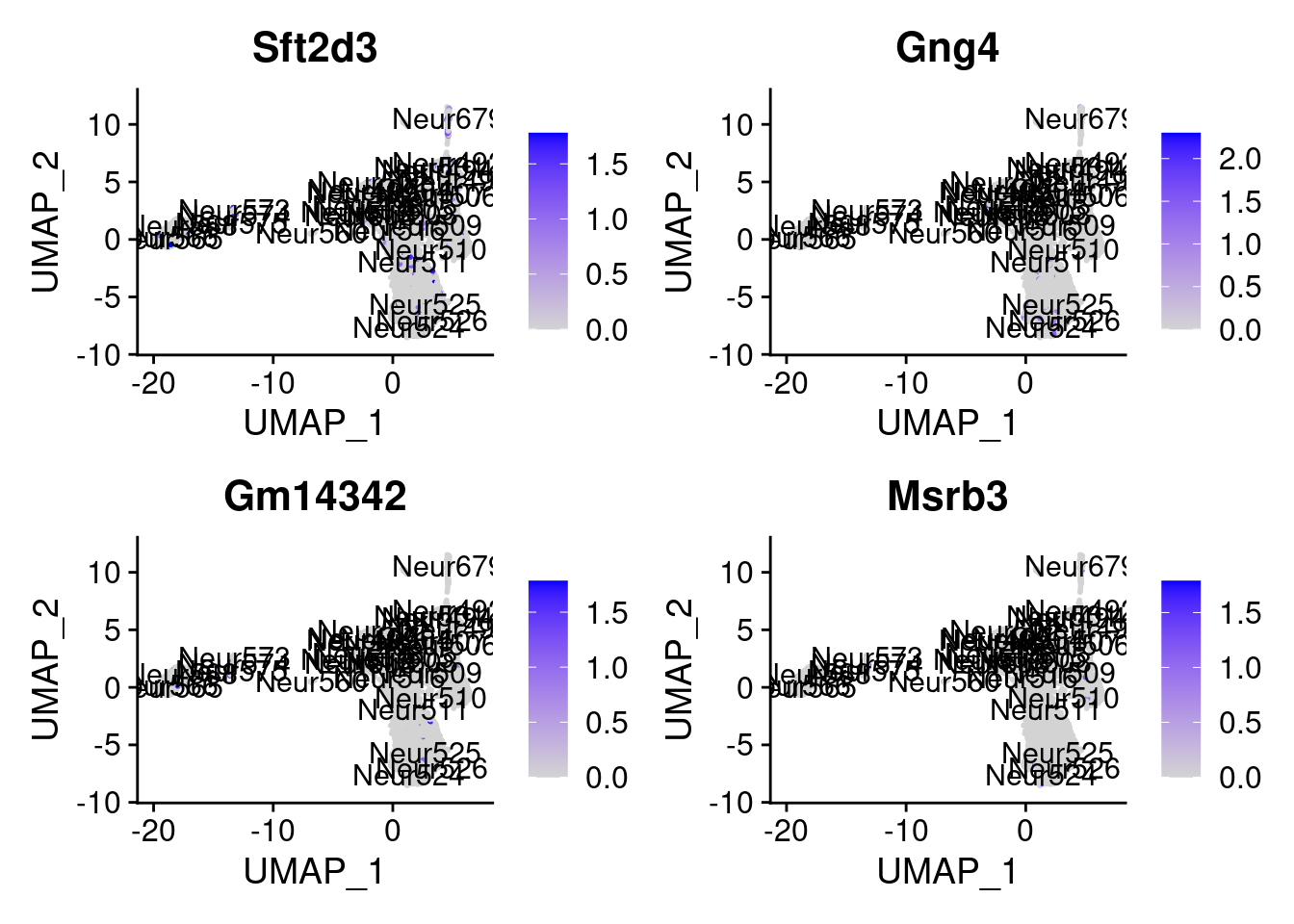
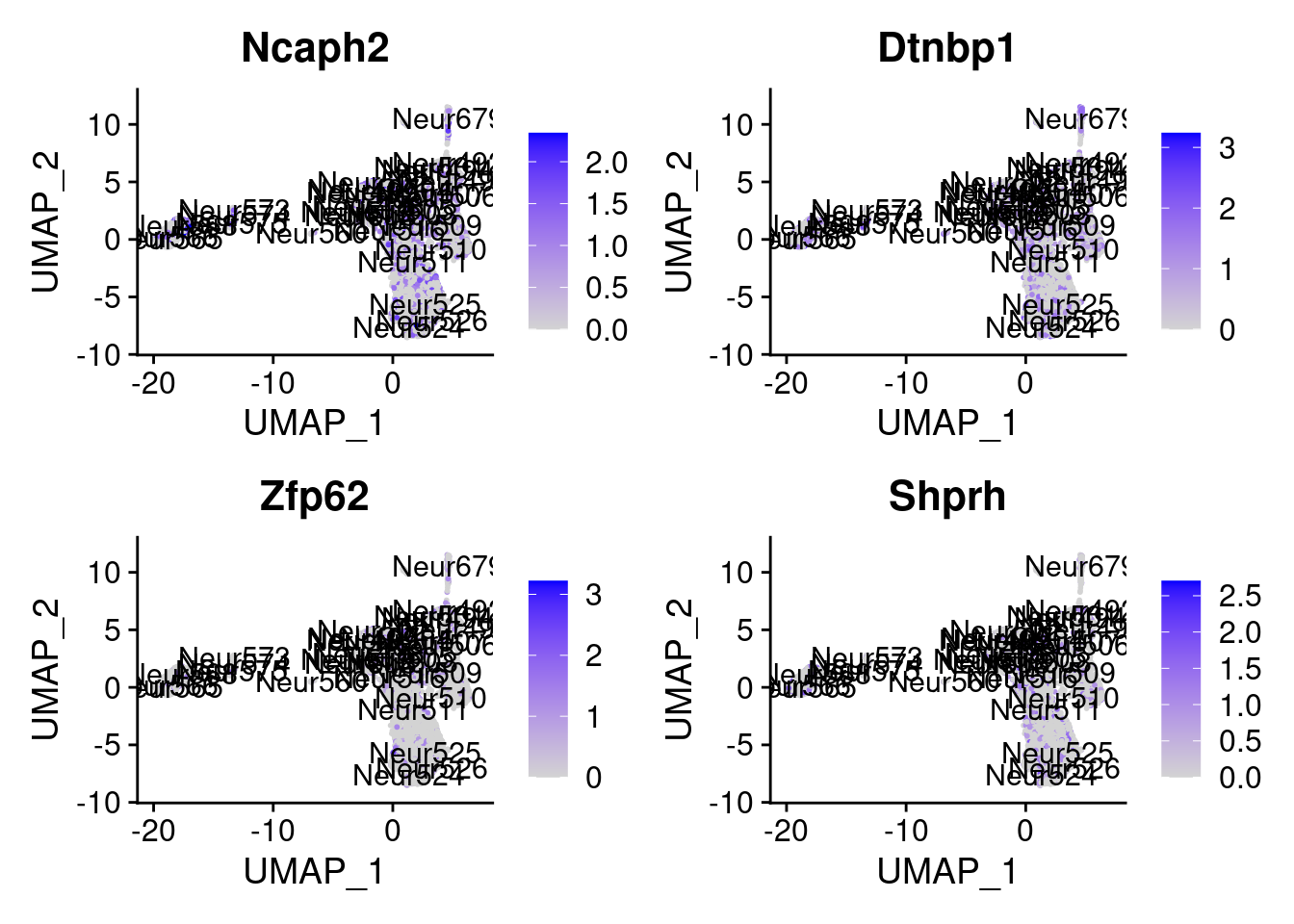
 [1] "Met"        "Rsbn1l"     "Zfp358"     "Enpp5"      "Sft2d3"
 [6] "Gng4"       "Gm14342"    "Msrb3"      "Ncaph2"     "Dtnbp1"
[11] "Zfp62"      "Shprh"      "Bmf"        "AC174678.1" "Map7d1"
[16] "Srsf1"      "Smim7"      "Rab39b"     "Depdc7"     "Prkg1"
[21] "Rad21"      "Brinp1"     "Rbm5"       "Laptm4b"    "Dcbld2"
[26] "Slf2"       "Fam173a"    "Sh3bp5l"    "Slc1a2"     "Sstr1"
= 0 for (g in c (0 : 2 )) {= g* 4 plot (FeaturePlot (seurat.obj,features = genes[n+ c (1 : 4 )], label = T))
<- getNumOfExpressingCells (fb150Obj)[genes.to.test.Cotan]<- as.data.frame (df)colnames (df) <- "CellNumber" rownames (df) <- NULL $ type <- "Only Cotan Genes" <- as.data.frame (getNumOfExpressingCells (fb150Obj)[sample (getGenes (fb150Obj), size = length (rownames (df)))])rownames (df.bk) <- NULL colnames (df.bk) <- "CellNumber" $ type <- "Whole dataset Genes" <- rbind (df,df.bk)<- ddply (df, "type" , summarise, grp.mean= mean (CellNumber))ggplot (df,aes (x= CellNumber,fill= type))+ scale_fill_manual (values= c ("#C69AFF" , "#56B4E9" ))+ geom_histogram (aes (y= ..density..), position= "identity" , alpha= 0.5 ,bins = 25 )+ xlim (0 ,4800 )+ geom_vline (data= mu, aes (xintercept= grp.mean, color= type),linetype= "dashed" )+ geom_density (alpha= 0.6 )+ scale_y_continuous (labels = percent, name = "percent" ) + theme_classic ()+ theme (legend.position= "bottom" )
<- enrichr (genes.to.test, dbs)
Uploading data to Enrichr... Done.
  Querying ARCHS4_Tissues... Done.
Parsing results... Done.
plotEnrich (enriched[[1 ]], showTerms = 10 , numChar = 40 , y = "Count" , orderBy = "P.value" )
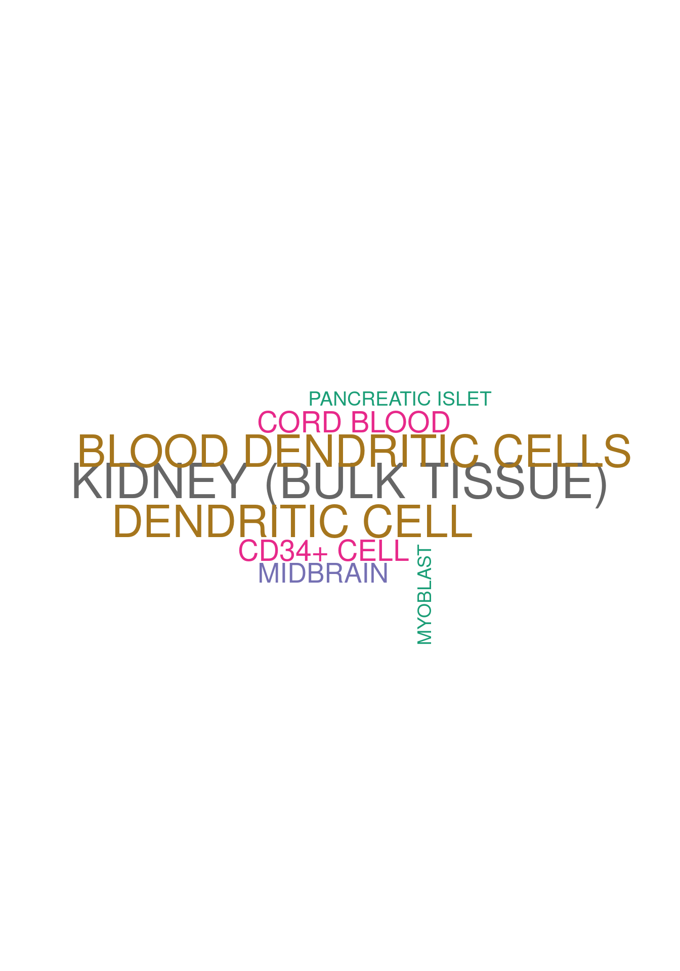
set.seed (12333 )<- data.frame (Terms = str_split (enriched[[1 ]]$ Term[1 : 5 ],pattern = " CL" ,simplify = T )[,1 ],Scores = enriched[[1 ]]$ Combined.Score[1 : 5 ])wordcloud (wordcloud_data$ Terms, wordcloud_data$ Scores, scale = c (3 , 1 ), min.freq = 1 , random.order= FALSE , rot.per= 0.1 ,colors= brewer.pal (8 , "Dark2" ))
<- dea.Subclass$ ` p-value ` [rownames (dea.Subclass$ ` p-value ` ) %in% genes.to.test.Cotan,]<- rownames (subset.pval[order (subset.pval$ ` Forebrain GABAergic ` ,decreasing = F),])[1 : length (genes.to.test)]<- enrichr (genes.to.test.Cotan.Top, dbs)
Uploading data to Enrichr... Done.
  Querying ARCHS4_Tissues... Done.
Parsing results... Done.
plotEnrich (enriched[[1 ]], showTerms = 10 , numChar = 40 , y = "Count" , orderBy = "P.value" )
set.seed (123 )<- data.frame (Terms = str_split (enriched[[1 ]]$ Term,pattern = " CL" ,simplify = T )[,1 ],Scores = enriched[[1 ]]$ Combined.Score)wordcloud (wordcloud_data$ Terms, wordcloud_data$ Scores, scale = c (3 , 1 ), min.freq = 1 , random.order= FALSE , rot.per= 0.1 ,colors= brewer.pal (8 , "Dark2" ))
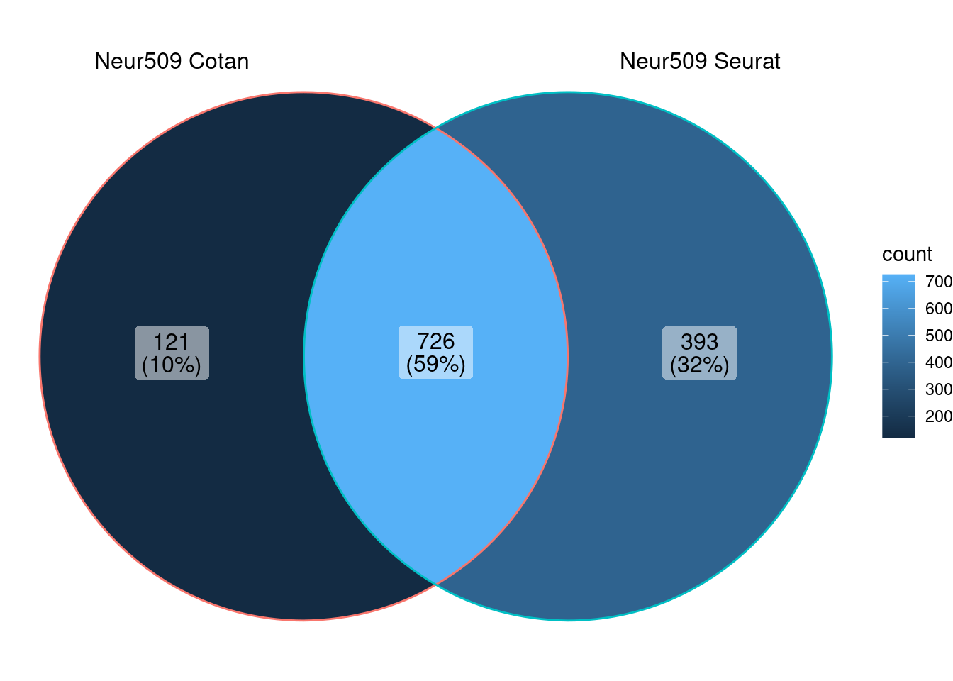
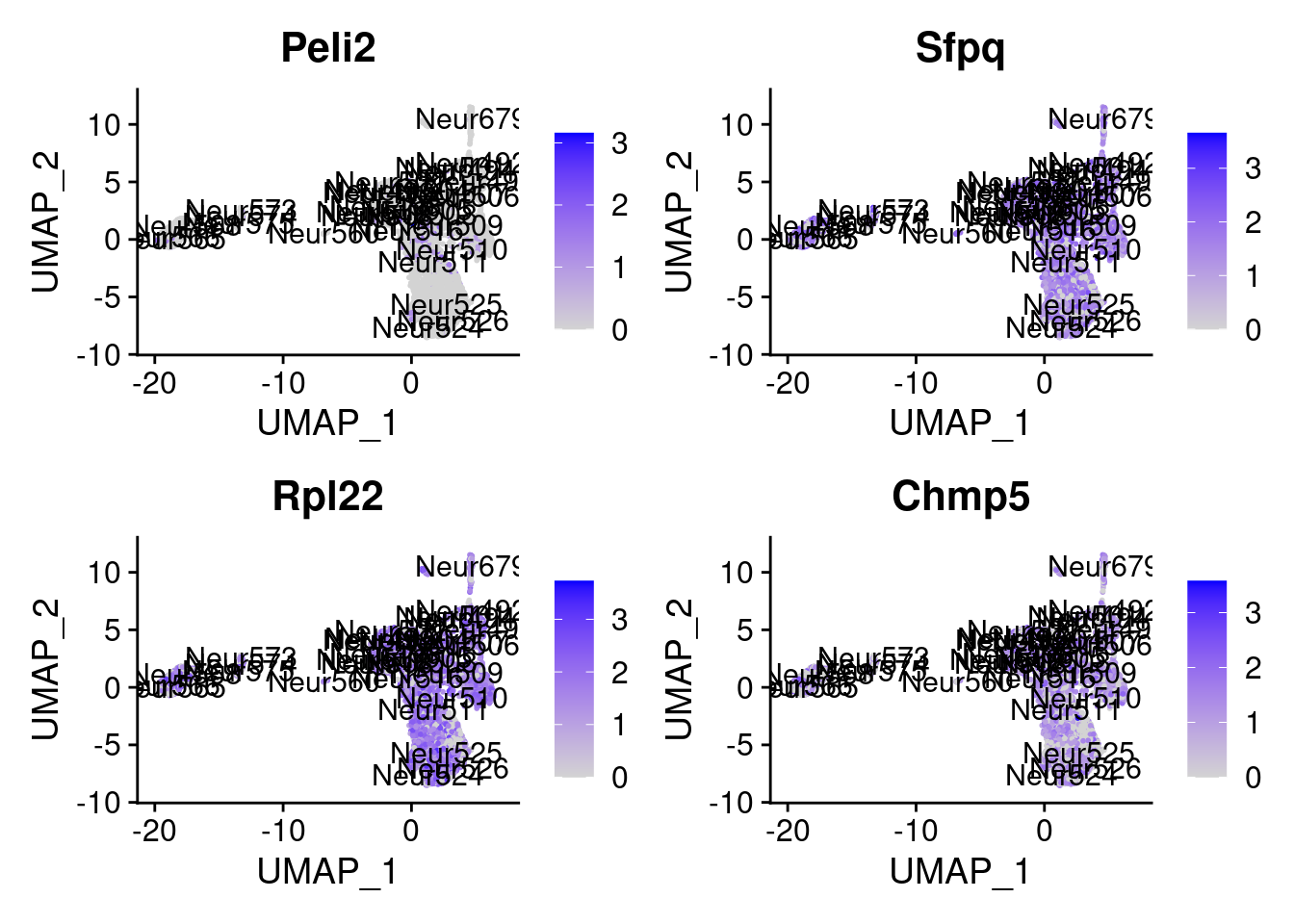
Cluster Neur509
# markers.list.namesNeur509 <- col_concat(crossing(colnames(dea.ClusterName$coex),c("Seurat","Cotan")),sep = " ") # # markers.listNeur509 <- vector("list", length(markers.list.namesNeur509)) # names(markers.listNeur509) <- markers.list.namesNeur509 <- list ("Neur509 Cotan" = NA ,"Neur509 Seurat" = NA )# I take positive coex significant genes for (cl.name in "Neur509" ) {<- rownames (dea.ClusterName$ coex[dea.ClusterName$ ` p-value ` [,cl.name] < 0.01 & dea.ClusterName$ coex[,cl.name] > 0 ,])paste0 (cl.name," Cotan" )]] <- genes#For seurat for (cl.name in "Neur509" ) {<- seurat.obj.markers.ClusterName[seurat.obj.markers.ClusterName$ cluster == cl.name & seurat.obj.markers.ClusterName$ p_val < 0.01 ,]$ genepaste0 (cl.name," Seurat" )]] <- genes
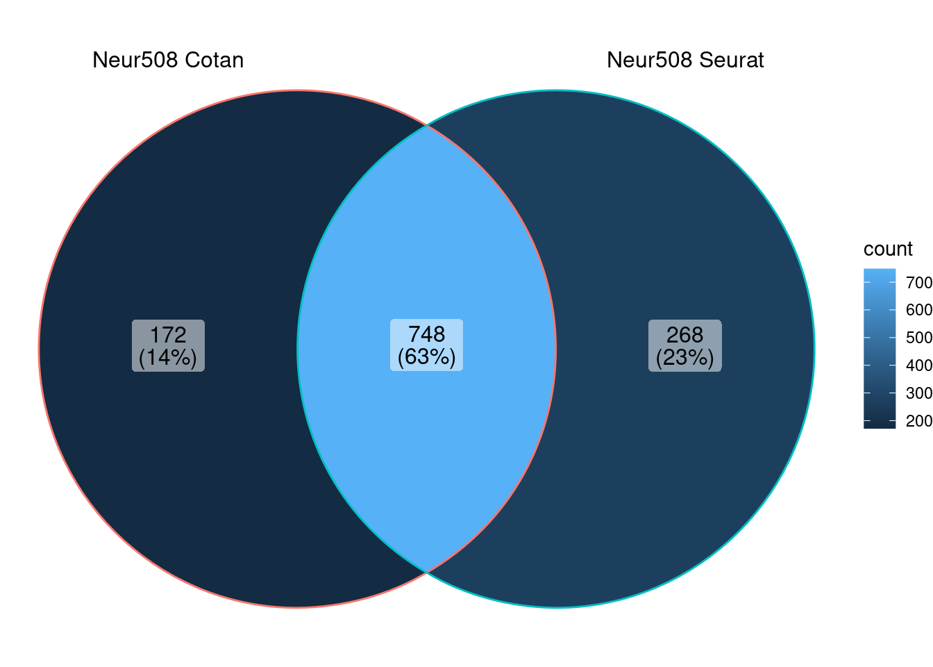
ggVennDiagram (markers.listNeur509)
We can observe that there is a good overlap among the detected markers.
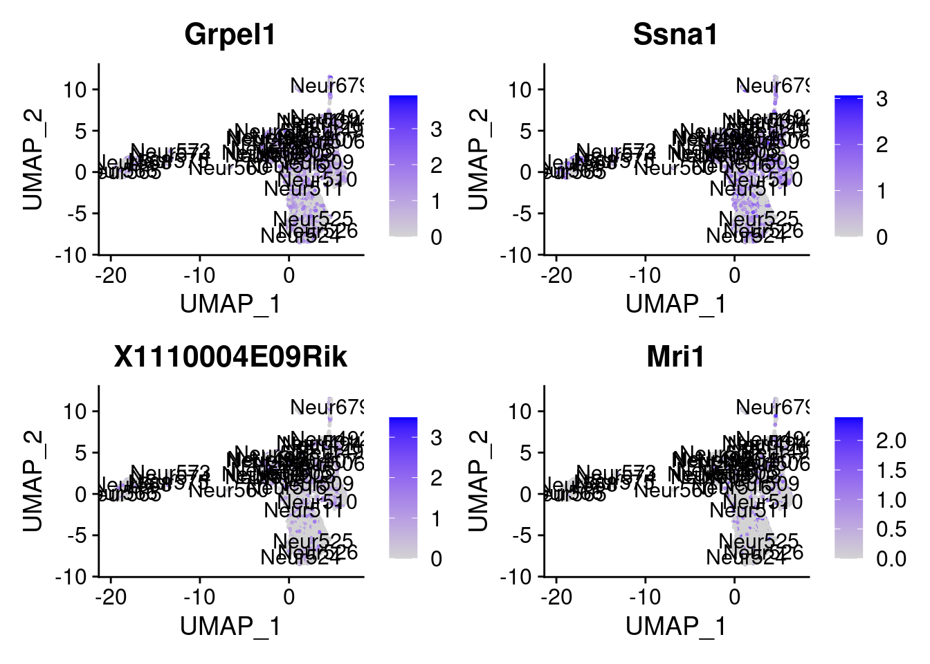
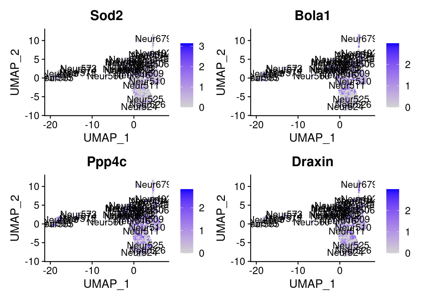
<- markers.listNeur509$ ` Neur509 Seurat ` [! markers.listNeur509$ ` Neur509 Seurat ` %in% markers.listNeur509$ ` Neur509 Cotan ` ]<- getNumOfExpressingCells (fb150Obj)[genes.to.test]<- as.data.frame (df)colnames (df) <- "CellNumber" rownames (df) <- NULL $ type <- "Only Seurat Genes" <- as.data.frame (getNumOfExpressingCells (fb150Obj)[sample (getGenes (fb150Obj), size = length (rownames (df)))])rownames (df.bk) <- NULL colnames (df.bk) <- "CellNumber" $ type <- "Whole dataset Genes" <- rbind (df,df.bk)<- ddply (df, "type" , summarise, grp.mean= mean (CellNumber))ggplot (df,aes (x= CellNumber,fill= type))+ scale_fill_manual (values= c ("#E69F00" , "#56B4E9" ))+ geom_histogram (aes (y= ..density..), position= "identity" , alpha= 0.5 ,bins = 25 )+ xlim (0 ,4800 )+ geom_vline (data= mu, aes (xintercept= grp.mean, color= type),linetype= "dashed" )+ geom_density (alpha= 0.6 )+ scale_y_continuous (labels = percent, name = "percent of genes" ) + theme_classic ()+ theme (legend.position= "bottom" )
set.seed (111 )<- sample (genes.to.test,size = 12 )
 [1] "Grpel1"         "Ssna1"          "X1110004E09Rik" "Mri1"
 [5] "Sod2"           "Bola1"          "Ppp4c"          "Draxin"
 [9] "Peli2"          "Sfpq"           "Rpl22"          "Chmp5"
= 0 for (g in c (0 : 2 )) {= g* 4 plot (FeaturePlot (seurat.obj,features = genes[n+ c (1 : 4 )], label = T))
Generally if we look at the genes specifically detected by Seurat, they don’t seems so distinctive for CR cells.
sum (genes.to.test %in% markers.listNeur509$ ` Cortical or hippocampal glutamatergic Seurat ` )/ length (genes.to.test)
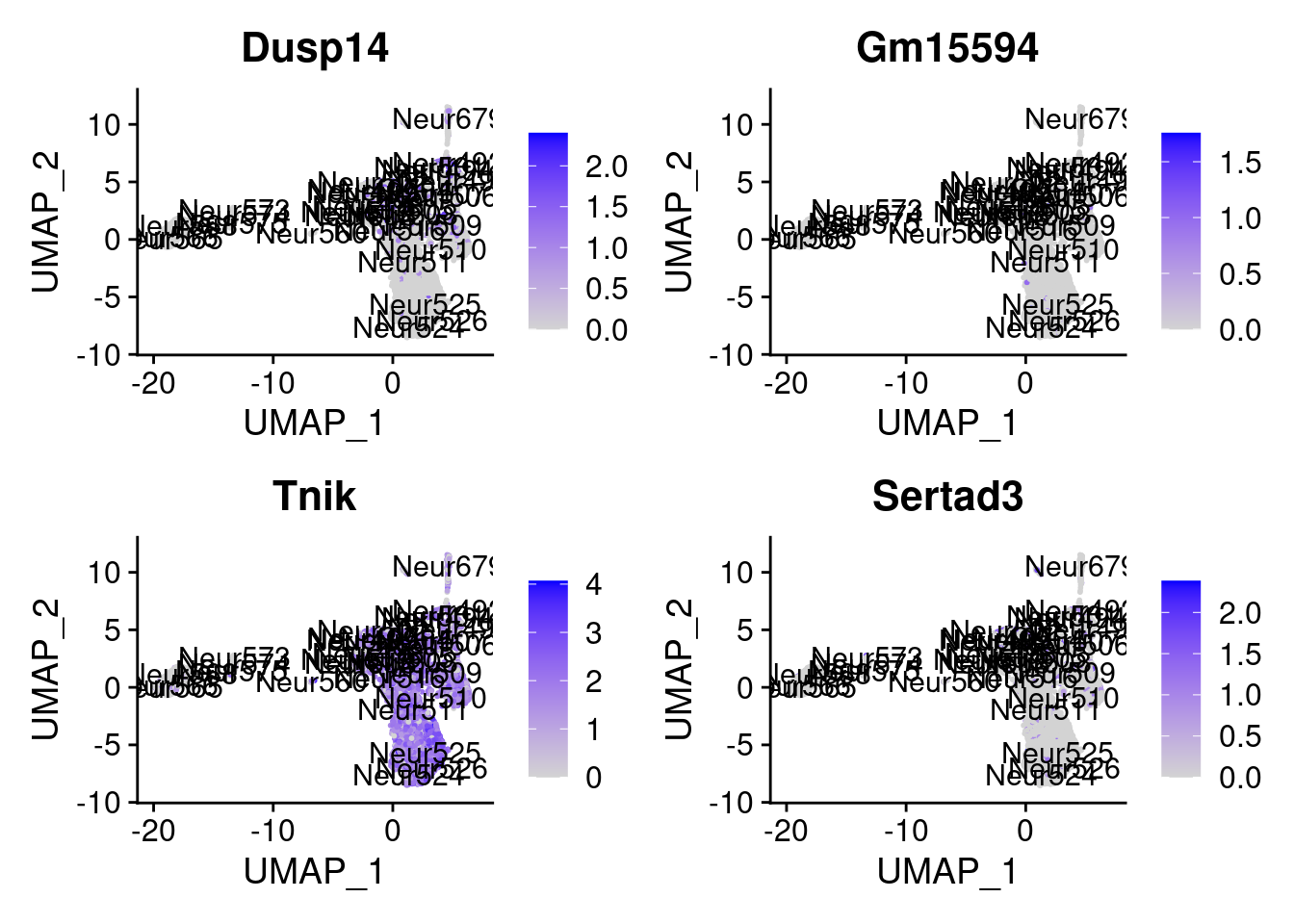
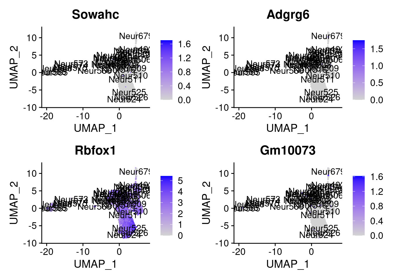
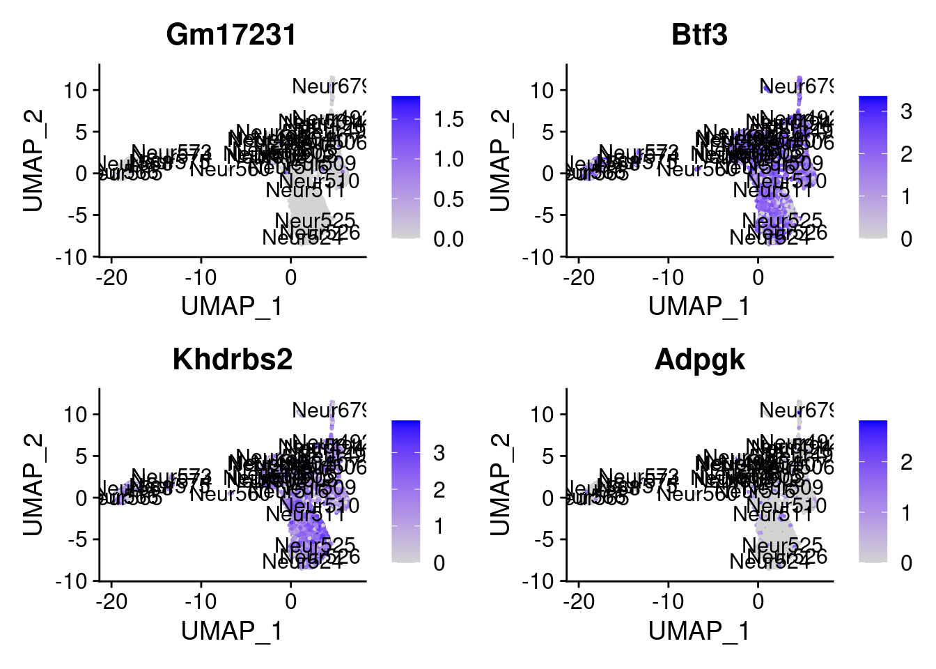
<- markers.listNeur509$ ` Neur509 Cotan ` [! markers.listNeur509$ ` Neur509 Cotan ` %in% markers.listNeur509$ ` Neur509 Seurat ` ]set.seed (11 )<- sample (genes.to.test.Cotan,size = 30 )
 [1] "Dusp14"     "Gm15594"    "Tnik"       "Sertad3"    "Sowahc"
 [6] "Adgrg6"     "Rbfox1"     "Gm10073"    "Gm17231"    "Btf3"
[11] "Khdrbs2"    "Adpgk"      "Pih1d2"     "Capzb"      "Cox6b1"
[16] "Chst5"      "Dcxr"       "Tfdp2"      "Plcxd2"     "Prss41"
[21] "Kcnq5"      "AC152827.1" "Atg4a"      "Fezf2"      "Gm15489"
[26] "Cth"        "Zbtb44"     "Sec61a1"    "Rbm12b1"    "Hk2"
= 0 for (g in c (0 : 2 )) {= g* 4 plot (FeaturePlot (seurat.obj,features = genes[n+ c (1 : 4 )], label = T))
<- getNumOfExpressingCells (fb150Obj)[genes.to.test.Cotan]<- as.data.frame (df)colnames (df) <- "CellNumber" rownames (df) <- NULL $ type <- "Only Cotan Genes" <- as.data.frame (getNumOfExpressingCells (fb150Obj)[sample (getGenes (fb150Obj), size = length (rownames (df)))])rownames (df.bk) <- NULL colnames (df.bk) <- "CellNumber" $ type <- "Whole dataset Genes" <- rbind (df,df.bk)<- ddply (df, "type" , summarise, grp.mean= mean (CellNumber))ggplot (df,aes (x= CellNumber,fill= type))+ scale_fill_manual (values= c ("#C69AFF" , "#56B4E9" ))+ geom_histogram (aes (y= ..density..), position= "identity" , alpha= 0.5 ,bins = 25 )+ xlim (0 ,4800 )+ geom_vline (data= mu, aes (xintercept= grp.mean, color= type),linetype= "dashed" )+ geom_density (alpha= 0.6 )+ scale_y_continuous (labels = percent, name = "percent" ) + theme_classic ()+ theme (legend.position= "bottom" )
Now we can test the enrichment for the specific gene both in Seurat and in Cotan.
To make a comparison more equal we select the same number of genes (depending on the smallest group)
<- seurat.obj.markers.ClusterName[seurat.obj.markers.ClusterName$ cluster == "Neur509" & seurat.obj.markers.ClusterName$ gene %in% genes.to.test,]$ gene[1 : length (genes.to.test.Cotan)]<- enrichr (genes.to.testTop, dbs)
Uploading data to Enrichr... Done.
  Querying ARCHS4_Tissues... Done.
Parsing results... Done.
plotEnrich (enriched[[1 ]], showTerms = 10 , numChar = 40 , y = "Count" , orderBy = "P.value" )
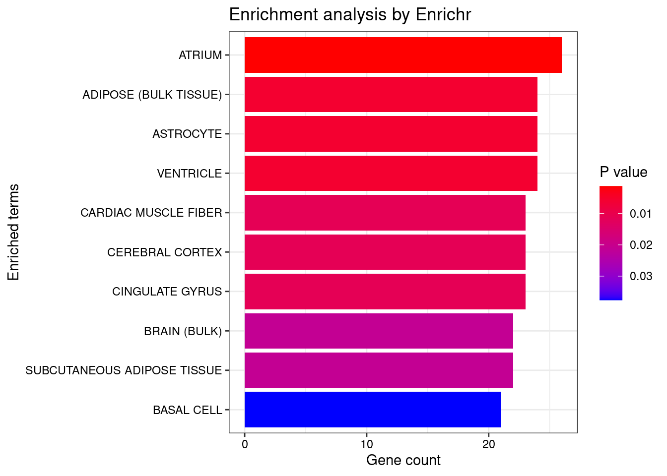
set.seed (123 )<- data.frame (Terms = str_split (enriched[[1 ]]$ Term[1 : 20 ],pattern = " CL" ,simplify = T )[,1 ],Scores = enriched[[1 ]]$ Combined.Score[1 : 20 ])wordcloud (wordcloud_data$ Terms, wordcloud_data$ Scores, scale = c (3 , 1 ), min.freq = 1 , random.order= FALSE , rot.per= 0.1 ,colors= brewer.pal (8 , "Dark2" ))
<- enrichr (genes.to.test.Cotan, dbs)
Uploading data to Enrichr... Done.
  Querying ARCHS4_Tissues... Done.
Parsing results... Done.
plotEnrich (enriched[[1 ]], showTerms = 10 , numChar = 40 , y = "Count" , orderBy = "P.value" )
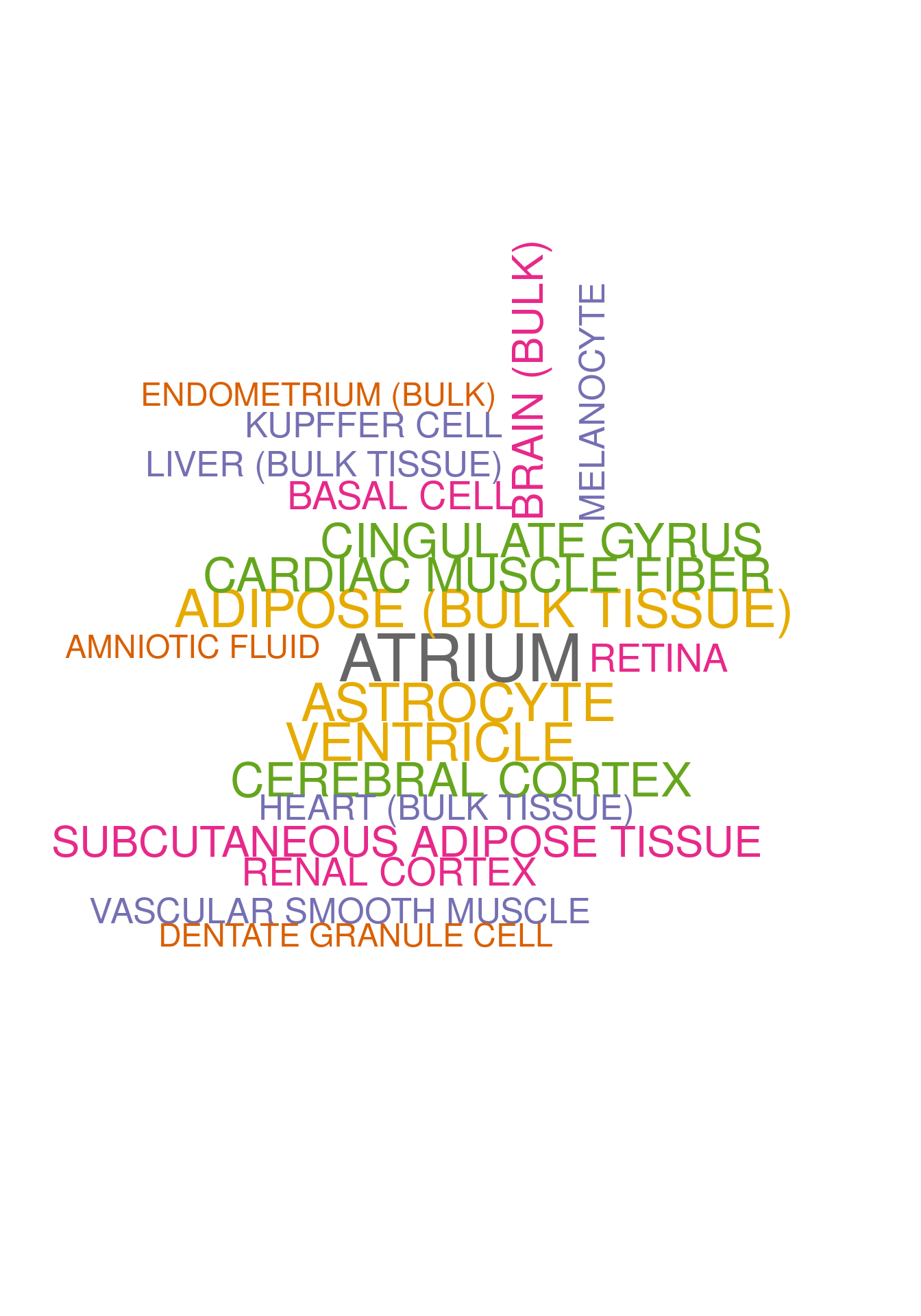
set.seed (123 )<- data.frame (Terms = str_split (enriched[[1 ]]$ Term[1 : 20 ],pattern = " CL" ,simplify = T )[,1 ],Scores = enriched[[1 ]]$ Combined.Score[1 : 20 ])wordcloud (wordcloud_data$ Terms, wordcloud_data$ Scores, scale = c (3 , 1 ), min.freq = 1 , random.order= FALSE , rot.per= 0.1 ,colors= brewer.pal (8 , "Dark2" ))
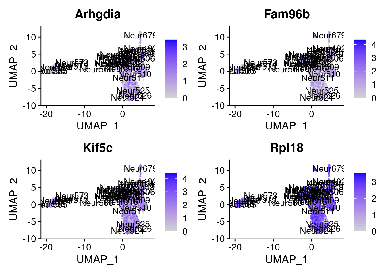
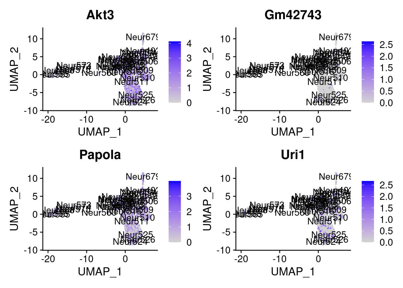
Cluster Neur508
# markers.list.namesNeur508 <- col_concat(crossing(colnames(dea.ClusterName$coex),c("Seurat","Cotan")),sep = " ") # # markers.listNeur508 <- vector("list", length(markers.list.namesNeur508)) # names(markers.listNeur508) <- markers.list.namesNeur508 <- list ("Neur508 Cotan" = NA ,"Neur508 Seurat" = NA )# I take positive coex significant genes for (cl.name in "Neur508" ) {<- rownames (dea.ClusterName$ coex[dea.ClusterName$ ` p-value ` [,cl.name] < 0.01 & dea.ClusterName$ coex[,cl.name] > 0 ,])paste0 (cl.name," Cotan" )]] <- genes#For seurat for (cl.name in "Neur508" ) {<- seurat.obj.markers.ClusterName[seurat.obj.markers.ClusterName$ cluster == cl.name & seurat.obj.markers.ClusterName$ p_val < 0.01 ,]$ genepaste0 (cl.name," Seurat" )]] <- genes
ggVennDiagram (markers.listNeur508)
We can observe that there is a good overlap among the detected markers.
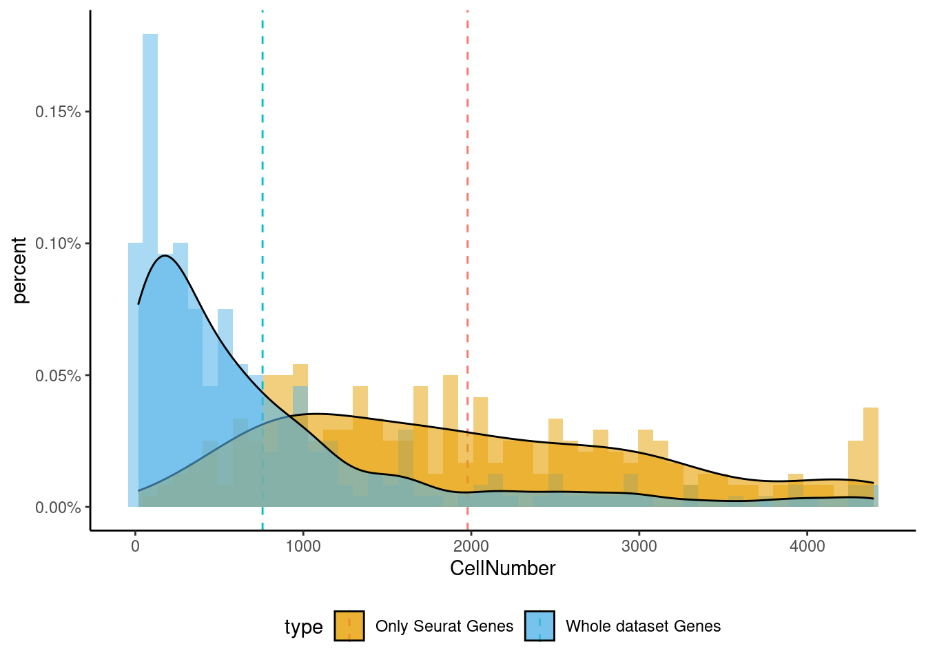
<- markers.listNeur508$ ` Neur508 Seurat ` [! markers.listNeur508$ ` Neur508 Seurat ` %in% markers.listNeur508$ ` Neur508 Cotan ` ]<- getNumOfExpressingCells (fb150Obj)[genes.to.test]<- as.data.frame (df)colnames (df) <- "CellNumber" rownames (df) <- NULL $ type <- "Only Seurat Genes" <- as.data.frame (getNumOfExpressingCells (fb150Obj)[sample (getGenes (fb150Obj), size = length (rownames (df)))])rownames (df.bk) <- NULL colnames (df.bk) <- "CellNumber" $ type <- "Whole dataset Genes" <- rbind (df,df.bk)<- ddply (df, "type" , summarise, grp.mean= mean (CellNumber))ggplot (df,aes (x= CellNumber,fill= type))+ scale_fill_manual (values= c ("#E69F00" , "#56B4E9" ))+ geom_histogram (aes (y= ..density..), position= "identity" , alpha= 0.5 ,bins = 50 )+ geom_vline (data= mu, aes (xintercept= grp.mean, color= type),linetype= "dashed" )+ geom_density (alpha= 0.6 )+ scale_y_continuous (labels = percent, name = "percent" ) + theme_classic ()+ theme (legend.position= "bottom" )
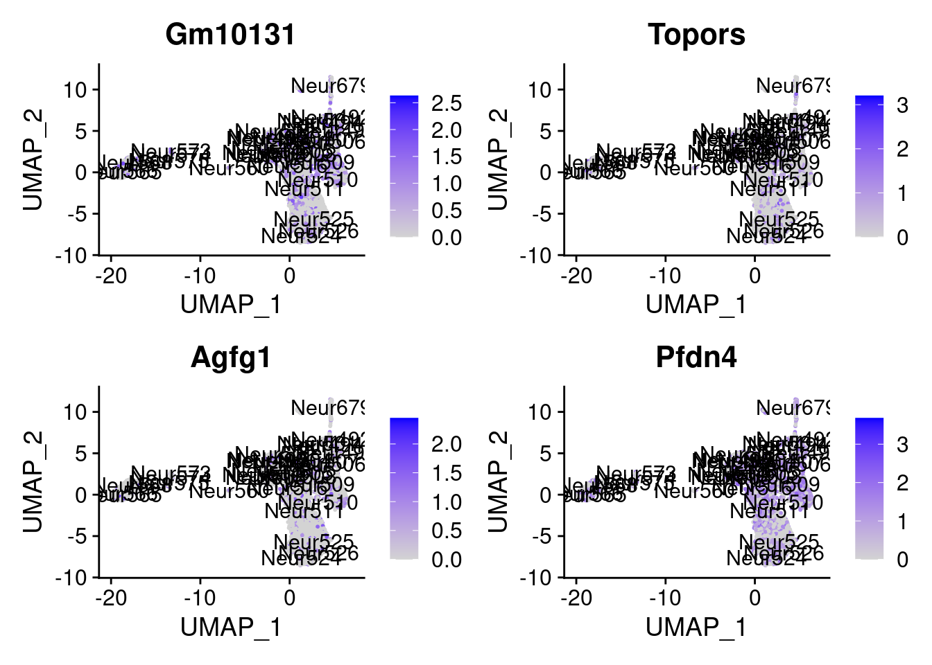
set.seed (111 )<- sample (genes.to.test,size = 12 )
 [1] "Gm10131" "Topors"  "Agfg1"   "Pfdn4"   "Arhgdia" "Fam96b"  "Kif5c"
 [8] "Rpl18"   "Akt3"    "Gm42743" "Papola"  "Uri1"
= 0 for (g in c (0 : 2 )) {= g* 4 plot (FeaturePlot (seurat.obj,features = genes[n+ c (1 : 4 )], label = T))
Generally if we look at the genes specifically detected by Seurat, they don’t seems so distinctive for CR cells.
sum (genes.to.test %in% markers.listNeur508$ ` Cortical or hippocampal glutamatergic Seurat ` )/ length (genes.to.test)
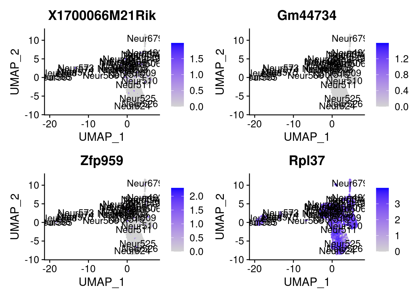
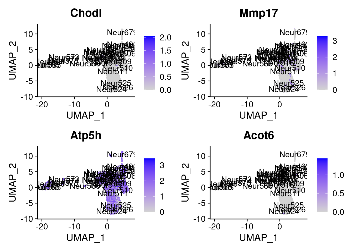
<- markers.listNeur508$ ` Neur508 Cotan ` [! markers.listNeur508$ ` Neur508 Cotan ` %in% markers.listNeur508$ ` Neur508 Seurat ` ]set.seed (11 )<- sample (genes.to.test.Cotan,size = 30 )
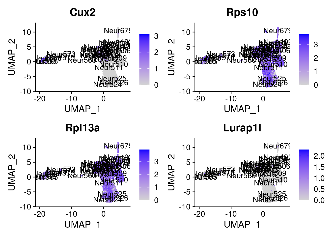
 [1] "X1700066M21Rik" "Gm44734"        "Zfp959"         "Rpl37"
 [5] "Chodl"          "Mmp17"          "Atp5h"          "Acot6"
 [9] "Cux2"           "Rps10"          "Rpl13a"         "Lurap1l"
[13] "Tcf12"          "Sirt6"          "Gm12184"        "Etohd2"
[17] "Laptm4b"        "Pomc"           "Rpl9"           "Inhbb"
[21] "Gpr62"          "Sstr3"          "D830035M03Rik"  "Eef1b2"
[25] "Bmpr1b"         "Rps4x"          "Tpd52"          "Selenow"
[29] "Pla2g7"         "Kcnj11"
= 0 for (g in c (0 : 2 )) {= g* 4 plot (FeaturePlot (seurat.obj,features = genes[n+ c (1 : 4 )], label = T))
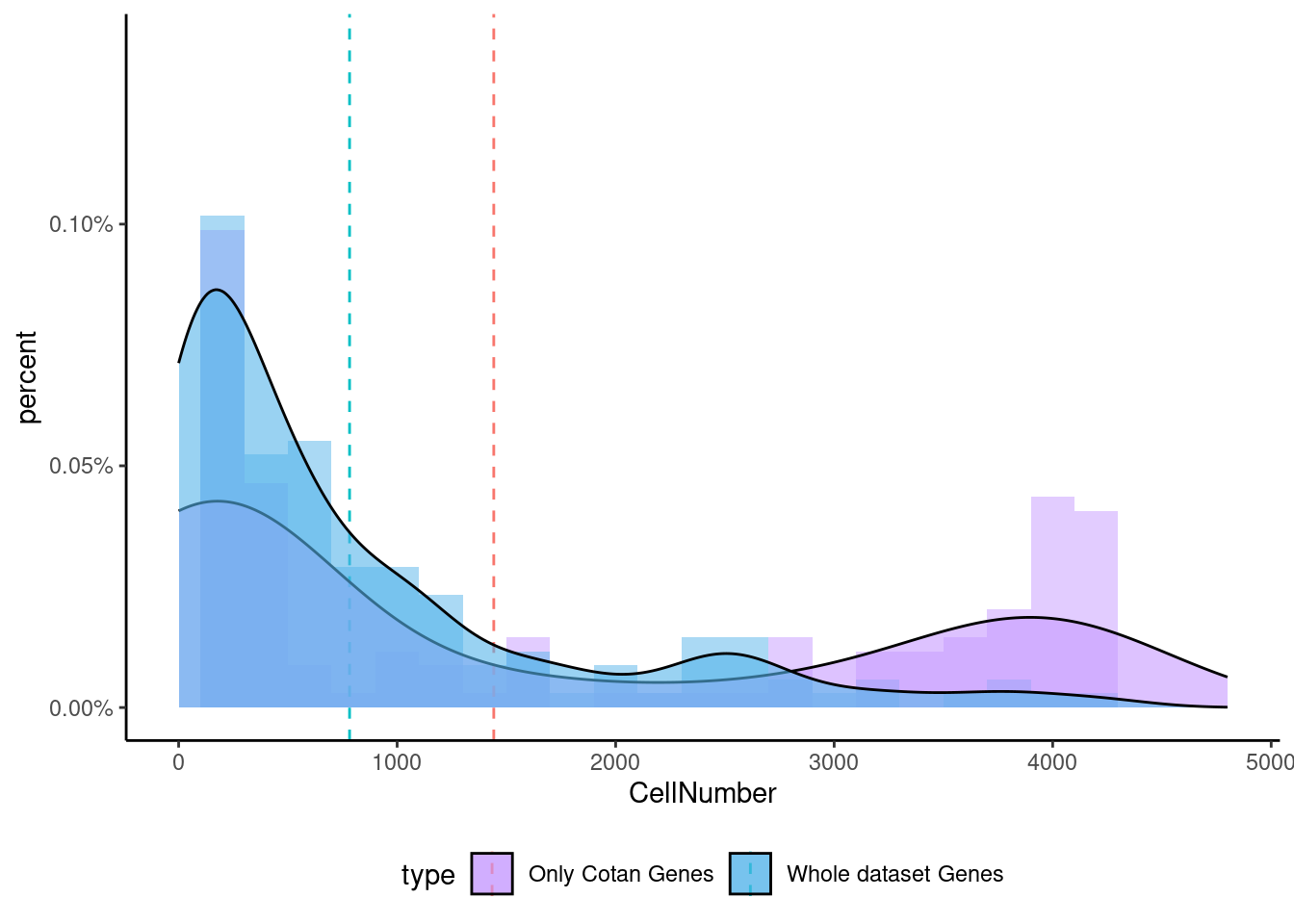
<- getNumOfExpressingCells (fb150Obj)[genes.to.test.Cotan]<- as.data.frame (df)colnames (df) <- "CellNumber" rownames (df) <- NULL $ type <- "Only Cotan Genes" <- as.data.frame (getNumOfExpressingCells (fb150Obj)[sample (getGenes (fb150Obj), size = length (rownames (df)))])rownames (df.bk) <- NULL colnames (df.bk) <- "CellNumber" $ type <- "Whole dataset Genes" <- rbind (df,df.bk)<- ddply (df, "type" , summarise, grp.mean= mean (CellNumber))ggplot (df,aes (x= CellNumber,fill= type))+ scale_fill_manual (values= c ("#C69AFF" , "#56B4E9" ))+ geom_histogram (aes (y= ..density..), position= "identity" , alpha= 0.5 ,bins = 25 )+ xlim (0 ,4800 )+ geom_vline (data= mu, aes (xintercept= grp.mean, color= type),linetype= "dashed" )+ geom_density (alpha= 0.6 )+ scale_y_continuous (labels = percent, name = "percent" ) + theme_classic ()+ theme (legend.position= "bottom" )
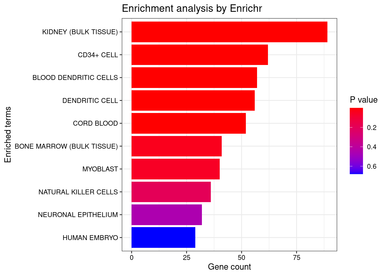
Now we can test the enrichment for the specific gene both in Seurat and in Cotan.
To make a comparison more equal we select the same number of genes (depending on the smallest group)
#genes.to.testTop <- seurat.obj.markers.ClusterName[seurat.obj.markers.ClusterName$cluster == "Neur508" & seurat.obj.markers.ClusterName$gene %in% genes.to.test,]$gene[1:length(genes.to.test.Cotan)] <- enrichr (genes.to.test, dbs)
Uploading data to Enrichr... Done.
  Querying ARCHS4_Tissues... Done.
Parsing results... Done.
plotEnrich (enriched[[1 ]], showTerms = 10 , numChar = 40 , y = "Count" , orderBy = "P.value" )
set.seed (123 )<- data.frame (Terms = str_split (enriched[[1 ]]$ Term[1 : 20 ],pattern = " CL" ,simplify = T )[,1 ],Scores = enriched[[1 ]]$ Combined.Score[1 : 20 ])wordcloud (wordcloud_data$ Terms, wordcloud_data$ Scores, scale = c (3 , 1 ), min.freq = 1 , random.order= FALSE , rot.per= 0.1 ,colors= brewer.pal (8 , "Dark2" ))
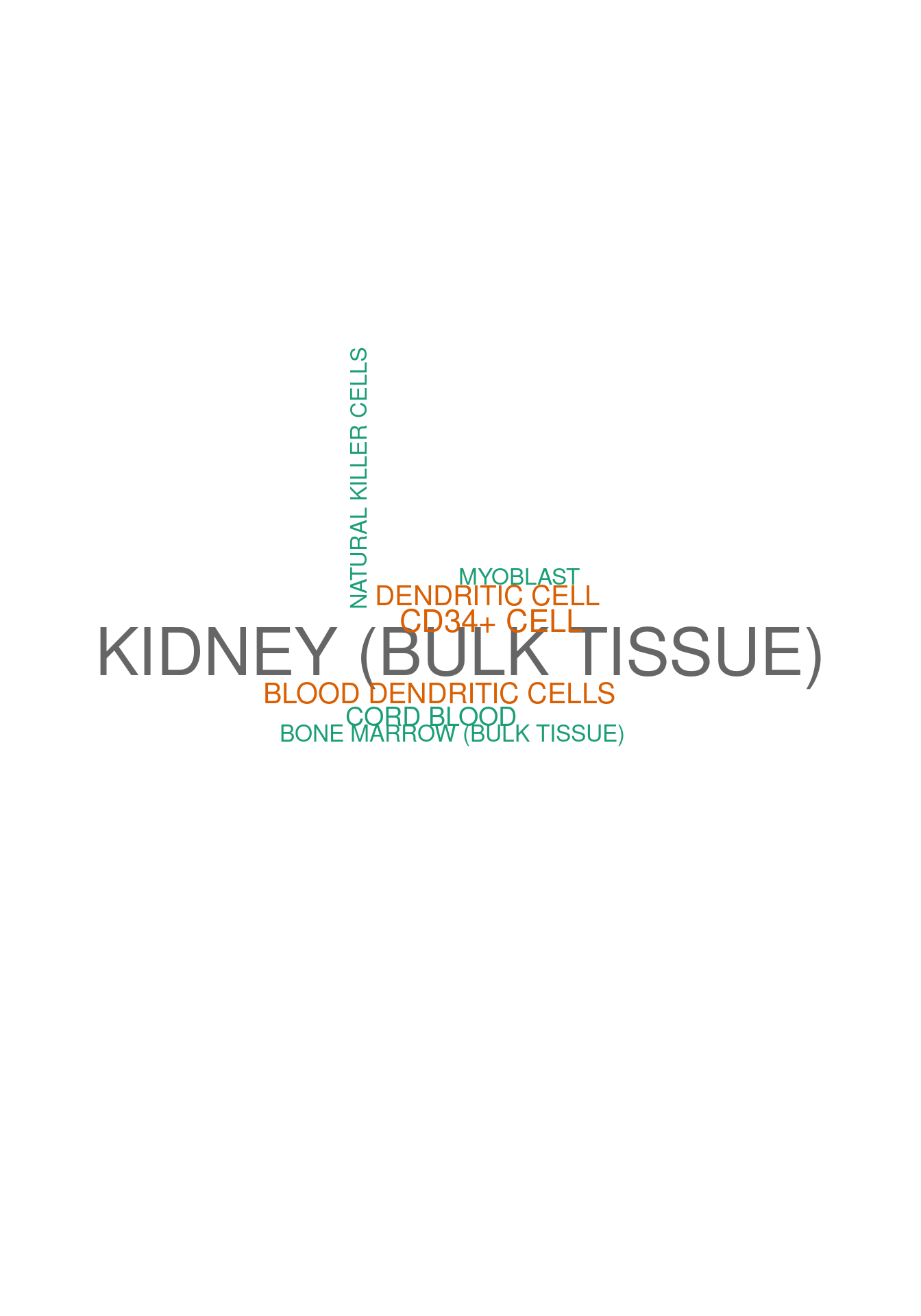
<- dea.ClusterName$ ` p-value ` [rownames (dea.ClusterName$ ` p-value ` ) %in% genes.to.test.Cotan,]<- rownames (subset.pval[order (subset.pval$ Neur492,decreasing = F),])[1 : length (genes.to.test)]<- enrichr (genes.to.test.Cotan.Top, dbs)
Uploading data to Enrichr... Done.
  Querying ARCHS4_Tissues... Done.
Parsing results... Done.
plotEnrich (enriched[[1 ]], showTerms = 10 , numChar = 40 , y = "Count" , orderBy = "P.value" )
set.seed (123 )<- data.frame (Terms = str_split (enriched[[1 ]]$ Term[1 : 20 ],pattern = " CL" ,simplify = T )[,1 ],Scores = enriched[[1 ]]$ Combined.Score[1 : 20 ])wordcloud (wordcloud_data$ Terms, wordcloud_data$ Scores, scale = c (3 , 1 ), min.freq = 1 , random.order= FALSE , rot.per= 0.1 ,colors= brewer.pal (8 , "Dark2" ))
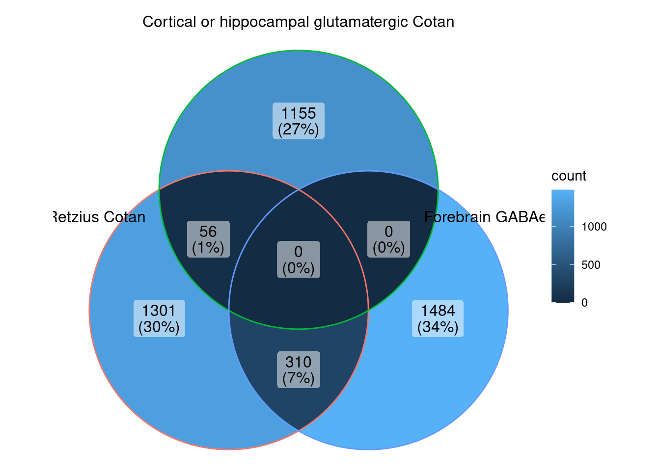
ggVennDiagram (markers.list[c (1 ,3 ,5 )])
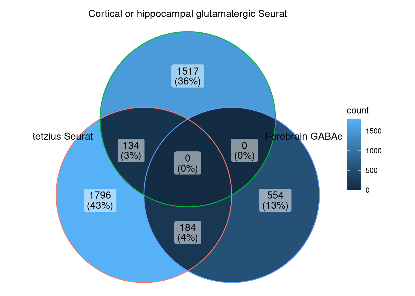
ggVennDiagram (markers.list[c (2 ,4 ,6 )])
R version 4.3.0 (2023-04-21)
Platform: x86_64-pc-linux-gnu (64-bit)
Running under: Ubuntu 20.04.6 LTS

Matrix products: default
BLAS:   /usr/lib/x86_64-linux-gnu/blas/libblas.so.3.9.0
LAPACK: /usr/lib/x86_64-linux-gnu/lapack/liblapack.so.3.9.0

locale:
 [1] LC_CTYPE=C.UTF-8       LC_NUMERIC=C           LC_TIME=C.UTF-8
 [4] LC_COLLATE=C.UTF-8     LC_MONETARY=C.UTF-8    LC_MESSAGES=C.UTF-8
 [7] LC_PAPER=C.UTF-8       LC_NAME=C              LC_ADDRESS=C
[10] LC_TELEPHONE=C         LC_MEASUREMENT=C.UTF-8 LC_IDENTIFICATION=C

time zone: Europe/Berlin
tzcode source: system (glibc)

attached base packages:
[1] stats     graphics  grDevices utils     datasets  methods   base

other attached packages:
 [1] enrichR_3.2         tidyr_1.3.0         ggVennDiagram_1.2.2
 [4] assertr_3.0.0       stringr_1.5.0       wordcloud_2.6
 [7] RColorBrewer_1.1-3  SeuratObject_4.1.3  Seurat_4.3.0
[10] rlang_1.1.0         scales_1.2.1        plyr_1.8.8
[13] COTAN_2.1.5         zeallot_0.1.0       tibble_3.2.1
[16] ggplot2_3.4.2

loaded via a namespace (and not attached):
  [1] RcppAnnoy_0.0.20       splines_4.3.0          later_1.3.0
  [4] polyclip_1.10-4        factoextra_1.0.7       lifecycle_1.0.3
  [7] sf_1.0-13              doParallel_1.0.17      globals_0.16.2
 [10] lattice_0.21-8         MASS_7.3-59            dendextend_1.17.1
 [13] magrittr_2.0.3         limma_3.56.0           plotly_4.10.1
 [16] rmarkdown_2.21         yaml_2.3.7             httpuv_1.6.9
 [19] sctransform_0.3.5      askpass_1.1            sp_1.6-0
 [22] spatstat.sparse_3.0-1  reticulate_1.30        cowplot_1.1.1
 [25] pbapply_1.7-0          DBI_1.1.3              abind_1.4-5
 [28] Rtsne_0.16             purrr_1.0.1            BiocGenerics_0.46.0
 [31] WriteXLS_6.4.0         circlize_0.4.15        IRanges_2.34.0
 [34] S4Vectors_0.38.0       ggrepel_0.9.3          irlba_2.3.5.1
 [37] listenv_0.9.0          spatstat.utils_3.0-3   units_0.8-2
 [40] umap_0.2.10.0          goftest_1.2-3          RSpectra_0.16-1
 [43] spatstat.random_3.1-4  fitdistrplus_1.1-8     parallelly_1.36.0
 [46] leiden_0.4.3           codetools_0.2-19       tidyselect_1.2.0
 [49] shape_1.4.6            farver_2.1.1           viridis_0.6.2
 [52] matrixStats_1.0.0      stats4_4.3.0           spatstat.explore_3.2-1
 [55] jsonlite_1.8.4         GetoptLong_1.0.5       e1071_1.7-13
 [58] ellipsis_0.3.2         progressr_0.13.0       ggridges_0.5.4
 [61] survival_3.5-5         iterators_1.0.14       foreach_1.5.2
 [64] tools_4.3.0            ica_1.0-3              Rcpp_1.0.10
 [67] glue_1.6.2             gridExtra_2.3          xfun_0.39
 [70] ggthemes_4.2.4         dplyr_1.1.2            withr_2.5.0
 [73] fastmap_1.1.1          fansi_1.0.4            openssl_2.0.6
 [76] digest_0.6.31          parallelDist_0.2.6     R6_2.5.1
 [79] mime_0.12              colorspace_2.1-0       scattermore_1.2
 [82] tensor_1.5             spatstat.data_3.0-1    utf8_1.2.3
 [85] generics_0.1.3         data.table_1.14.8      class_7.3-21
 [88] httr_1.4.5             htmlwidgets_1.6.2      uwot_0.1.14
 [91] pkgconfig_2.0.3        gtable_0.3.3           ComplexHeatmap_2.16.0
 [94] lmtest_0.9-40          htmltools_0.5.5        clue_0.3-64
 [97] png_0.1-8              knitr_1.42             rstudioapi_0.14
[100] reshape2_1.4.4         rjson_0.2.21           nlme_3.1-162
[103] curl_5.0.0             proxy_0.4-27           zoo_1.8-12
[106] GlobalOptions_0.1.2    RVenn_1.1.0            KernSmooth_2.23-20
[109] parallel_4.3.0         miniUI_0.1.1.1         vipor_0.4.5
[112] RcppZiggurat_0.1.6     ggrastr_1.0.2          pillar_1.9.0
[115] grid_4.3.0             vctrs_0.6.1            RANN_2.6.1
[118] promises_1.2.0.1       xtable_1.8-4           cluster_2.1.4
[121] beeswarm_0.4.0         evaluate_0.20          cli_3.6.1
[124] compiler_4.3.0         crayon_1.5.2           future.apply_1.11.0
[127] labeling_0.4.2         classInt_0.4-9         ggbeeswarm_0.7.2
[130] stringi_1.7.12         viridisLite_0.4.1      deldir_1.0-6
[133] assertthat_0.2.1       munsell_0.5.0          lazyeval_0.2.2
[136] spatstat.geom_3.2-1    Matrix_1.5-4.1         patchwork_1.1.2
[139] future_1.32.0          shiny_1.7.4            ROCR_1.0-11
[142] Rfast_2.0.7            igraph_1.4.2           RcppParallel_5.1.7