# Util libs
library(assertthat)
library(ggplot2)
library(zeallot)
library(conflicted)
library(Matrix)

# Data processing libs
if (!suppressWarnings(require(COTAN))) {
  devtools::load_all("~/dev/COTAN/COTAN/")
}

conflicts_prefer(zeallot::`%->%`, zeallot::`%<-%`)

options(parallelly.fork.enable = TRUE)

setLoggingLevel(2L)DatasetCleaning_Run77
Preamble
List input files
inDir <- file.path("..")
outDir <- file.path(".")

list.files(path = inDir, pattern = "\\.RDS$")
[1] "capillary_blood_samples_pbmcs-Run_28.RDS"
[2] "capillary_blood_samples_pbmcs-Run_40-Cleaned.RDS"
[3] "capillary_blood_samples_pbmcs-Run_40.RDS"
[4] "capillary_blood_samples_pbmcs-Run_41-Cleaned.RDS"
[5] "capillary_blood_samples_pbmcs-Run_41.RDS"
[6] "capillary_blood_samples_pbmcs-Run_62.RDS"
[7] "capillary_blood_samples_pbmcs-Run_77-Cleaned.RDS"
[8] "capillary_blood_samples_pbmcs-Run_77.RDS"
[9] "capillary_blood_samples_pbmcs.RDS" globalCondition <- "capillary_blood_samples_pbmcs"
thisRun <- "77"
fileNameIn <- paste0(globalCondition, "-Run_", thisRun, ".RDS")
setLoggingFile(file.path(outDir, paste0("DatasetCleaning_Run", thisRun, ".log")))Load dataset
aRunObj <- readRDS(file = file.path(inDir, fileNameIn))

getAllConditions(aRunObj)
[1] "Sample.IDs" "Participant.IDs"
[3] "Cell.Barcoding.Runs" "Lane"
[5] "cell_barcoding_protocol" "run_lane_batch"
[7] "original_sample_id" getClusterizations(aRunObj)[1] "cell_type_level_1" "cell_type_level_2" "cell_type_level_3"
[4] "cell_type_level_4" "c1" "c2"
[7] "c3" "c4" Cleaning
clean() using standard thresholds
Compare to the other runs, this one does not have the cell labelling!
#cellsToDrop <- names(getClusterizationData(aRunObj,"c4")[[1]][is.na(getClusterizationData(aRunObj,"c4")[[1]])])

#aRunObj <- dropGenesCells(aRunObj, cells = cellsToDrop)


aRunObj <- clean(aRunObj)
Check the initial plots
cellSizePlot(aRunObj, condName = "Participant.IDs")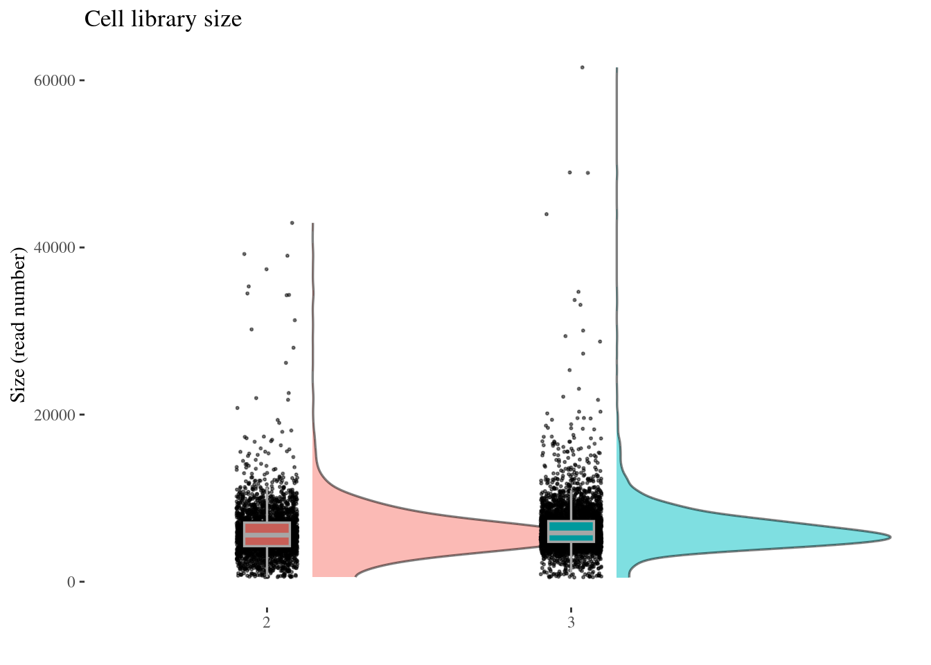
genesSizePlot(aRunObj, condName = "Participant.IDs")
scatterPlot(aRunObj, condName = "Participant.IDs")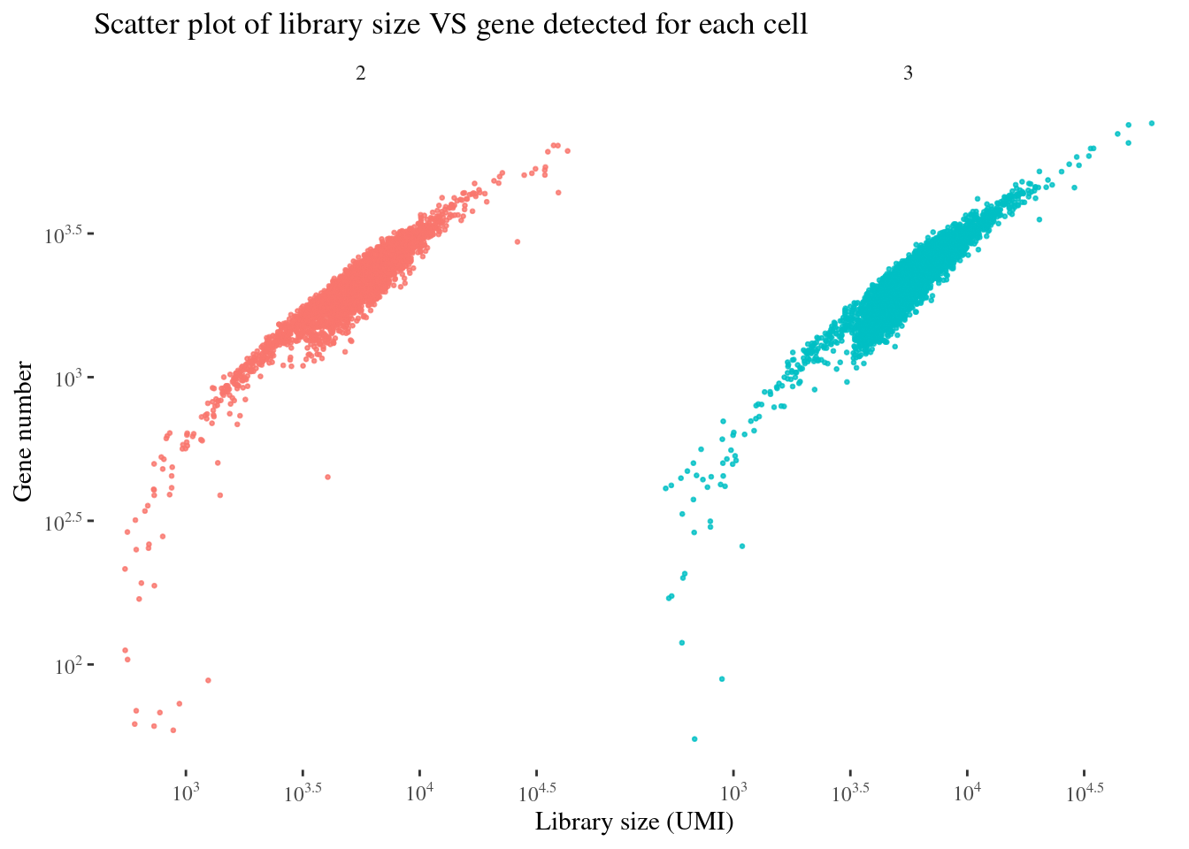
c(mitPerPlot, mitPerDf) %<-%
  mitochondrialPercentagePlot(aRunObj, condName = "Participant.IDs",
                              genePrefix = "^MT-")
mitPerPlot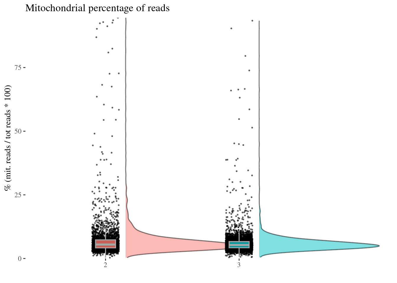
Remove too high mitochondrial percentage cells
Expected percentages are around 6%-10%: too high percentage imply dead cells
sum(mitPerDf[["mit.percentage"]] > 20.0)[1] 126sum(mitPerDf[["mit.percentage"]] > 15.0)[1] 219sum(mitPerDf[["mit.percentage"]] > 14.0)[1] 250sum(mitPerDf[["mit.percentage"]] > 10.0)[1] 537# drop above 14%
mitPerThr <- 20.0
aRunObj <-
addElementToMetaDataset(
aRunObj,
"Mitochondrial percentage threshold", mitPerThr)
cellsToDrop <- getCells(aRunObj)[which(mitPerDf[["mit.percentage"]] > mitPerThr)]
aRunObj <- dropGenesCells(aRunObj, cells = cellsToDrop)Redo the plots
cellSizePlot(aRunObj, condName = "Participant.IDs")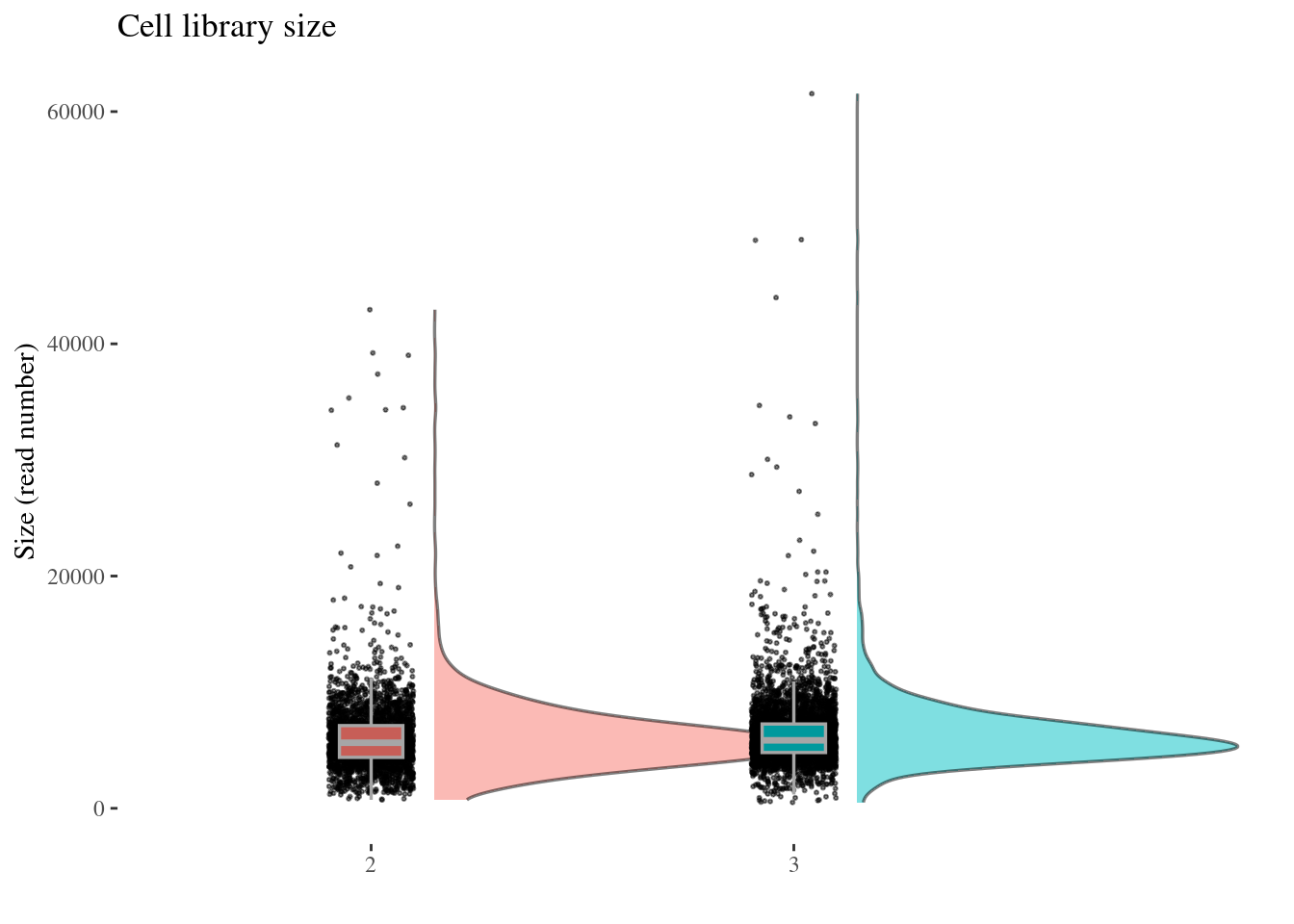
genesSizePlot(aRunObj, condName = "Participant.IDs")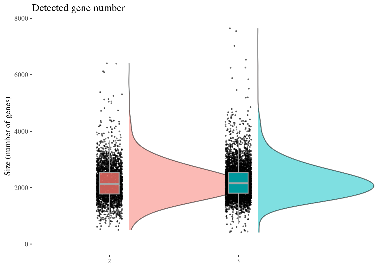
scatterPlot(aRunObj, condName = "Participant.IDs")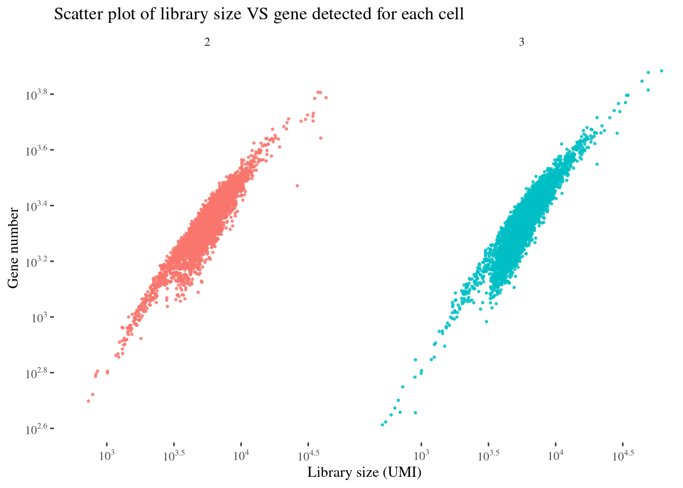
c(mitPerPlot, mitPerDf) %<-%
  mitochondrialPercentagePlot(aRunObj, condName = "Participant.IDs",
                              genePrefix = "^MT-")
mitPerPlot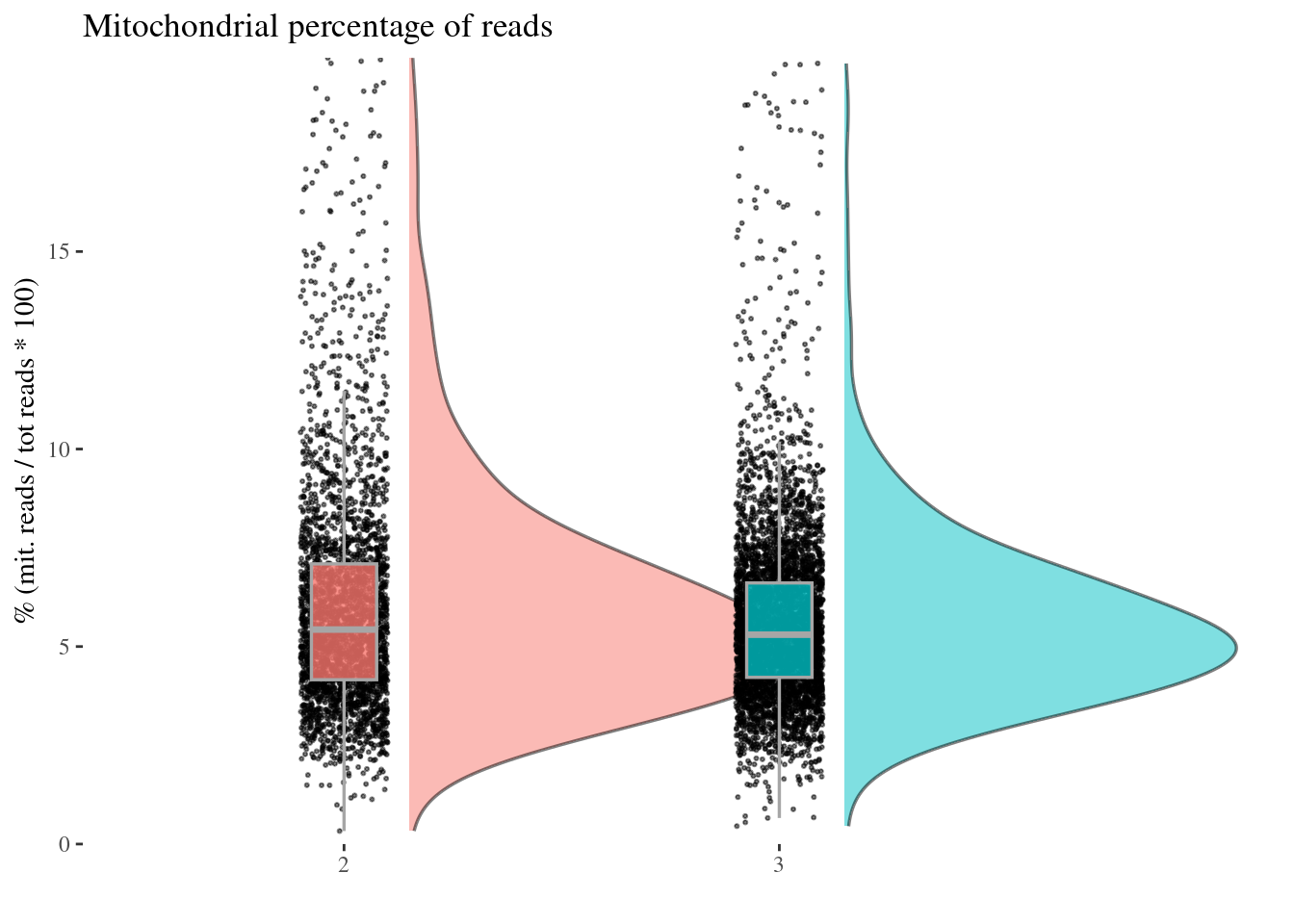
Remove cells with too high size
librarySize <- getCellsSize(aRunObj)

sum(librarySize > 25000)
[1] 24sum(librarySize > 20000)[1] 34sum(librarySize > 18000)[1] 47sum(librarySize > 15000)[1] 99sum(librarySize > 14000)[1] 118# drop above 15K
cellSizeThr <- 15000
aRunObj <-
addElementToMetaDataset(
aRunObj,
"Cell size threshold", cellSizeThr)
cellsToDrop <- getCells(aRunObj)[which(librarySize > cellSizeThr)]
aRunObj <- dropGenesCells(aRunObj, cells = cellsToDrop)Redo the plots
cellSizePlot(aRunObj, condName = "Participant.IDs")
genesSizePlot(aRunObj, condName = "Participant.IDs")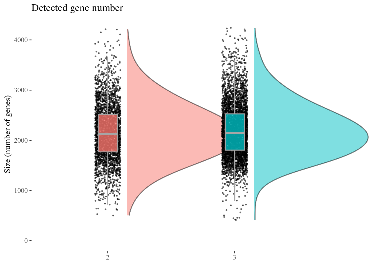
scatterPlot(aRunObj, condName = "Participant.IDs")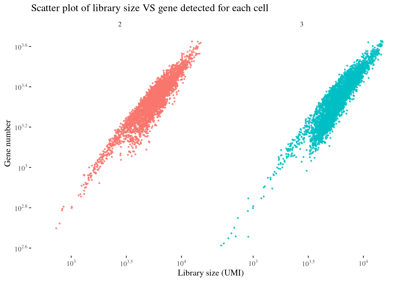
c(mitPerPlot, mitPerDf) %<-%
  mitochondrialPercentagePlot(aRunObj, condName = "Participant.IDs",
                              genePrefix = "^MT-")
mitPerPlot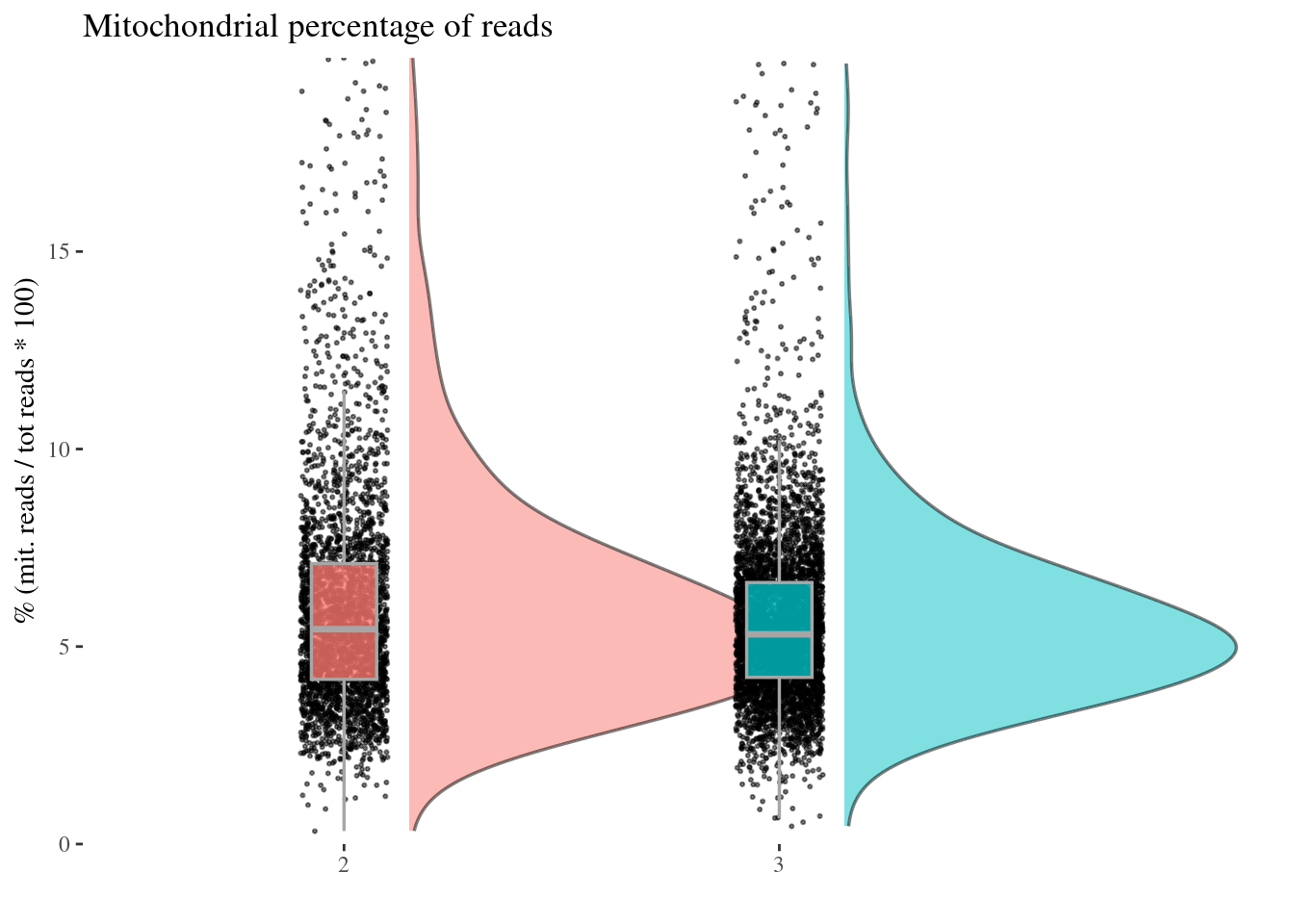
Check for spurious clusters
aRunObj <- clean(aRunObj)

c(pcaCells, pcaCellsData, genes, UDE, nu, zoomedNu) %<-%
  cleanPlots(aRunObj, includePCA = TRUE)
Plot PCA and Nu
plot(pcaCells)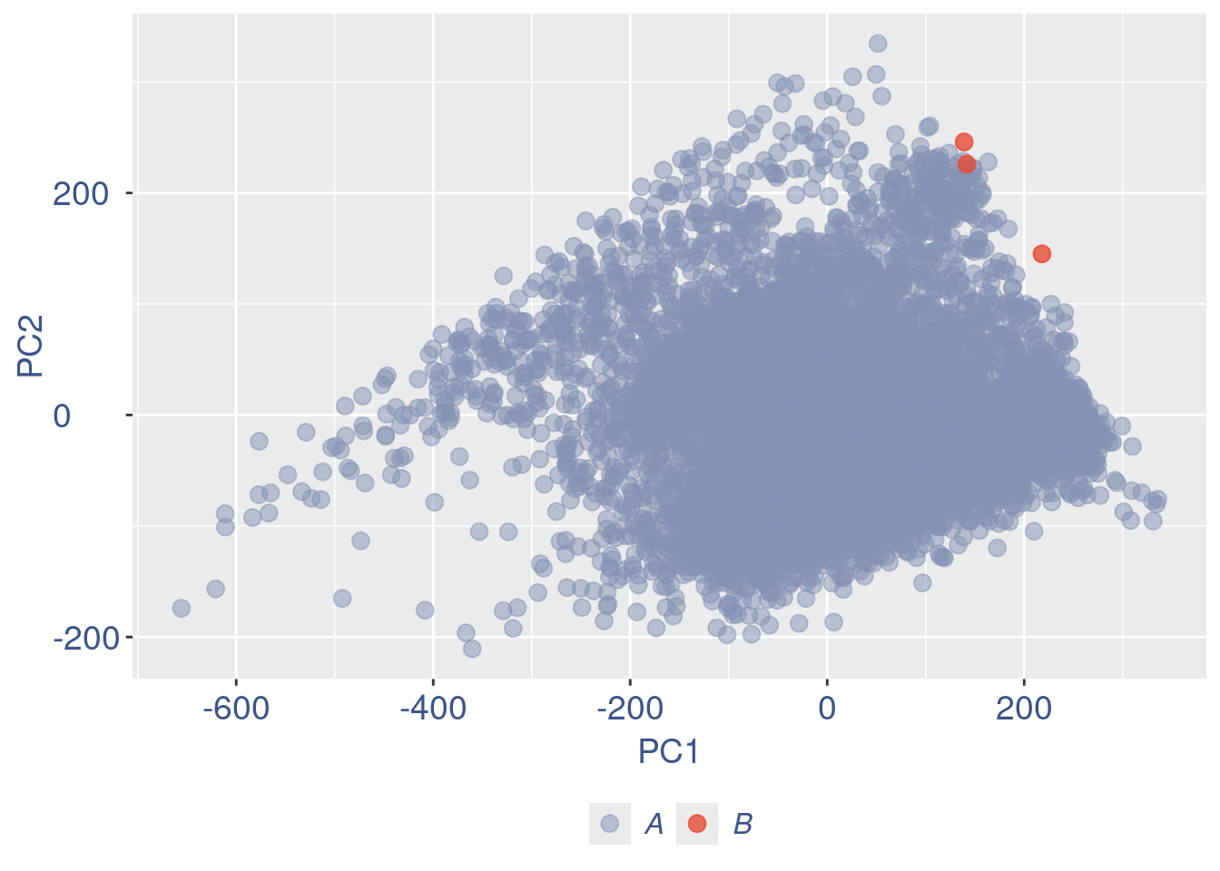
plot(UDE)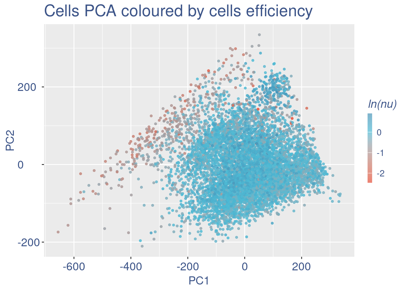
plot(pcaCellsData)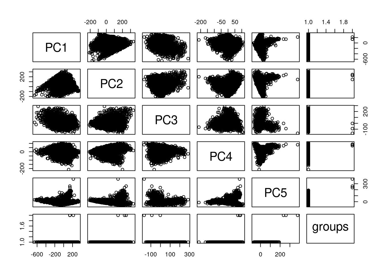
plot(genes)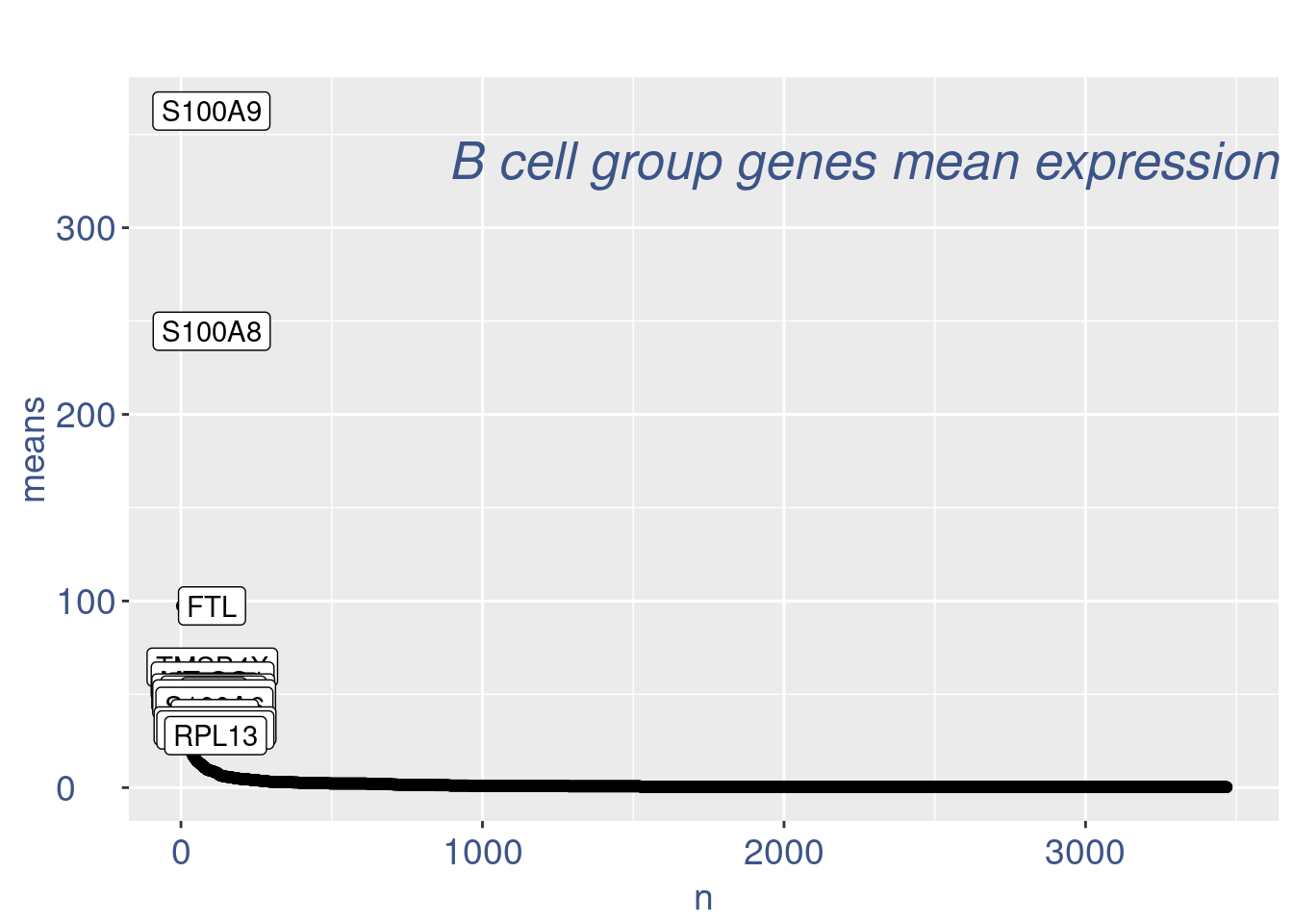
plot(nu)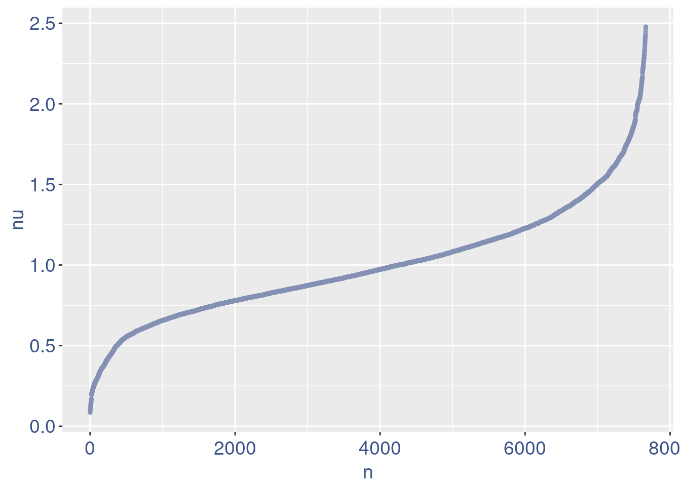
plot(zoomedNu)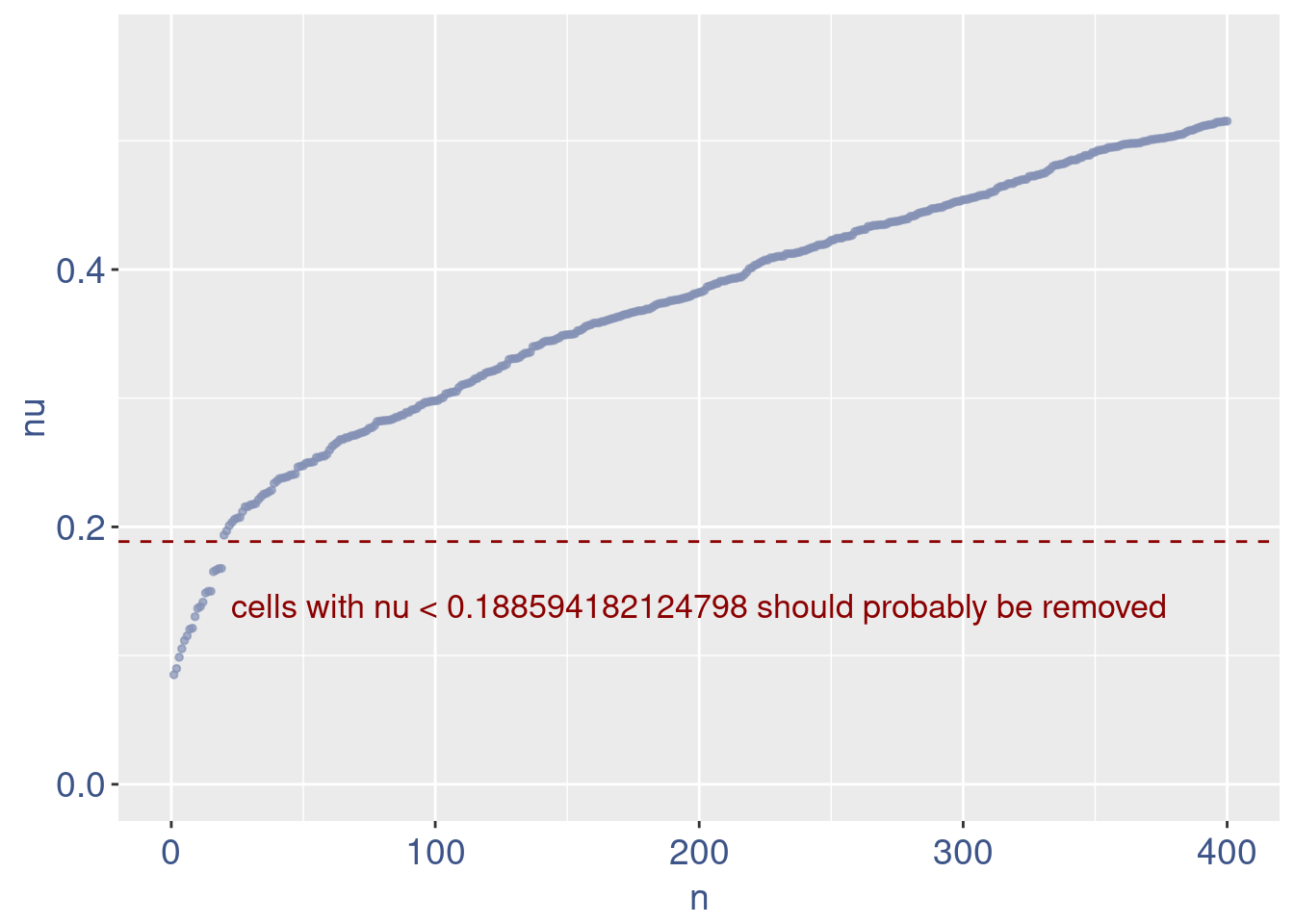
Remove cells below nu elbow point
nu <- getNu(aRunObj)

sum(nu < 0.15)
[1] 15sum(nu < 0.18)[1] 19sum(nu < 0.20)[1] 21# drop above 11%
lowNuThr <- 0.19
aRunObj <-
addElementToMetaDataset(
aRunObj,
"Low Nu threshold", lowNuThr)
cellsToDrop <- getCells(aRunObj)[which(nu < lowNuThr)]
cells_to_rem <- rownames(pcaCellsData)[pcaCellsData[["groups"]] == "B"]
aRunObj <- dropGenesCells(aRunObj, cells = c(cellsToDrop,cells_to_rem))Redo all the plots
aRunObj <- clean(aRunObj)

c(pcaCells, pcaCellsData, genes, UDE, nu, zoomedNu) %<-%
cleanPlots(aRunObj, includePCA = TRUE)plot(pcaCells)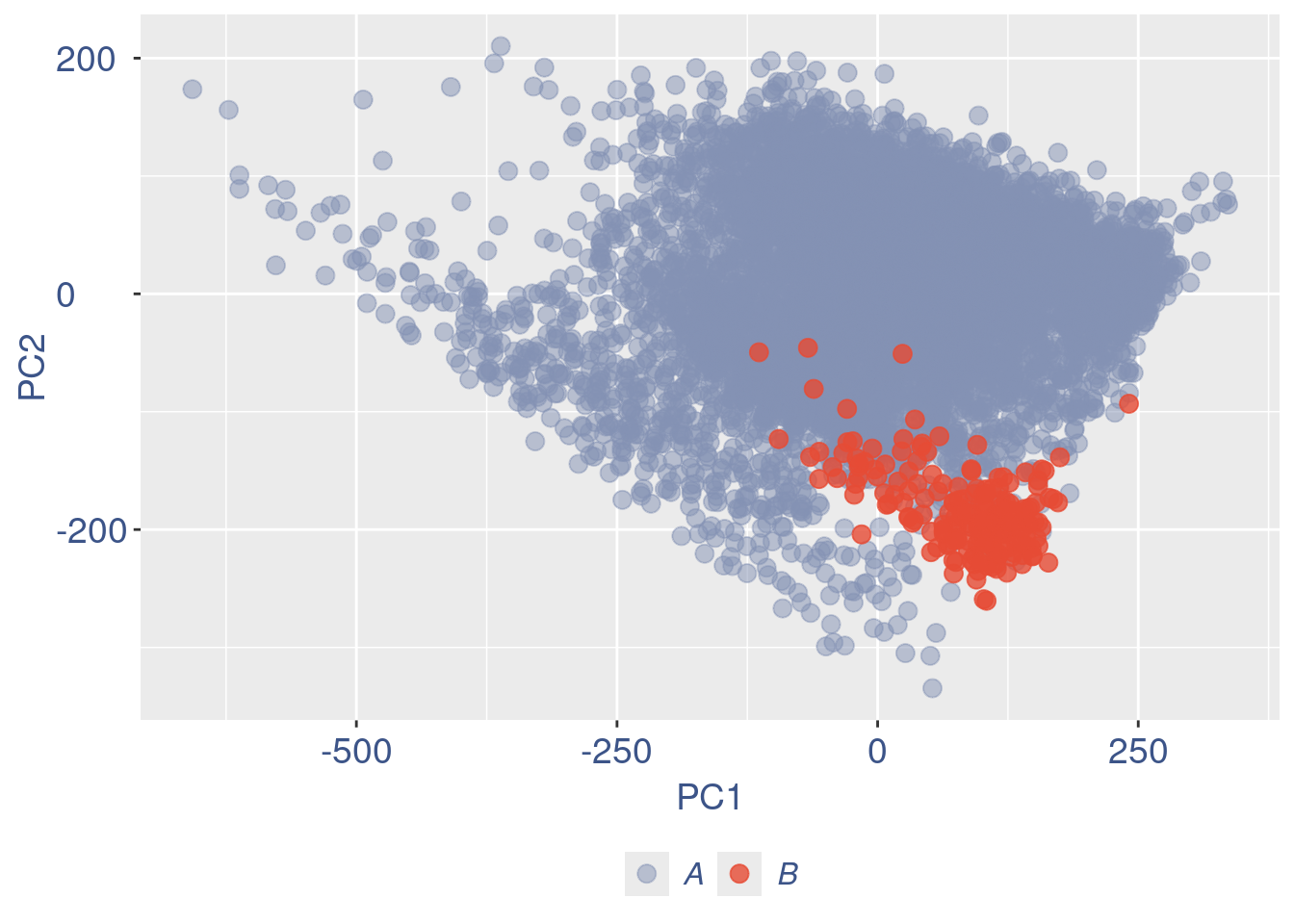
plot(UDE)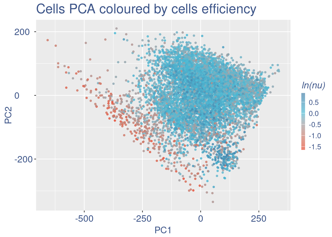
plot(pcaCellsData)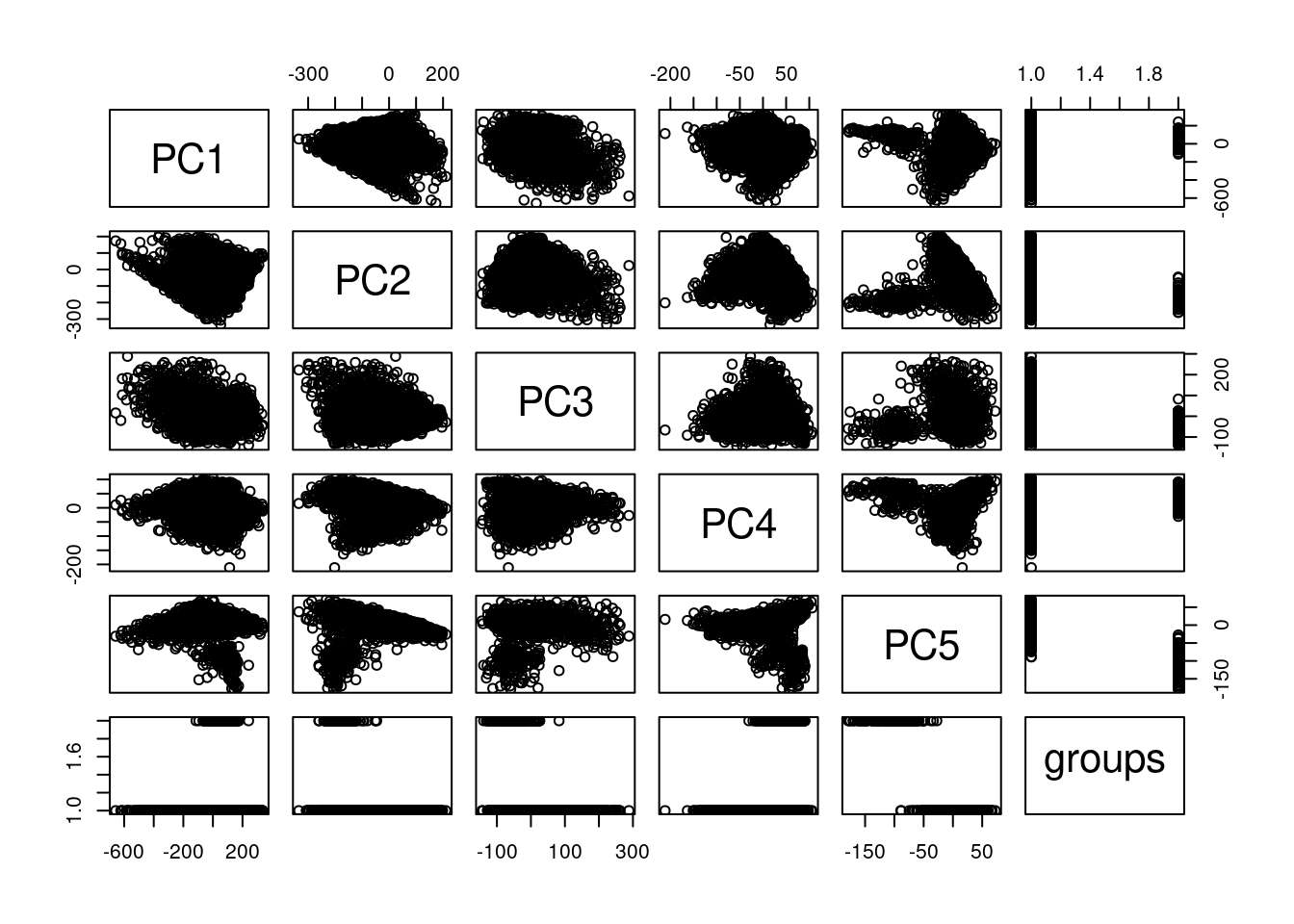
plot(genes)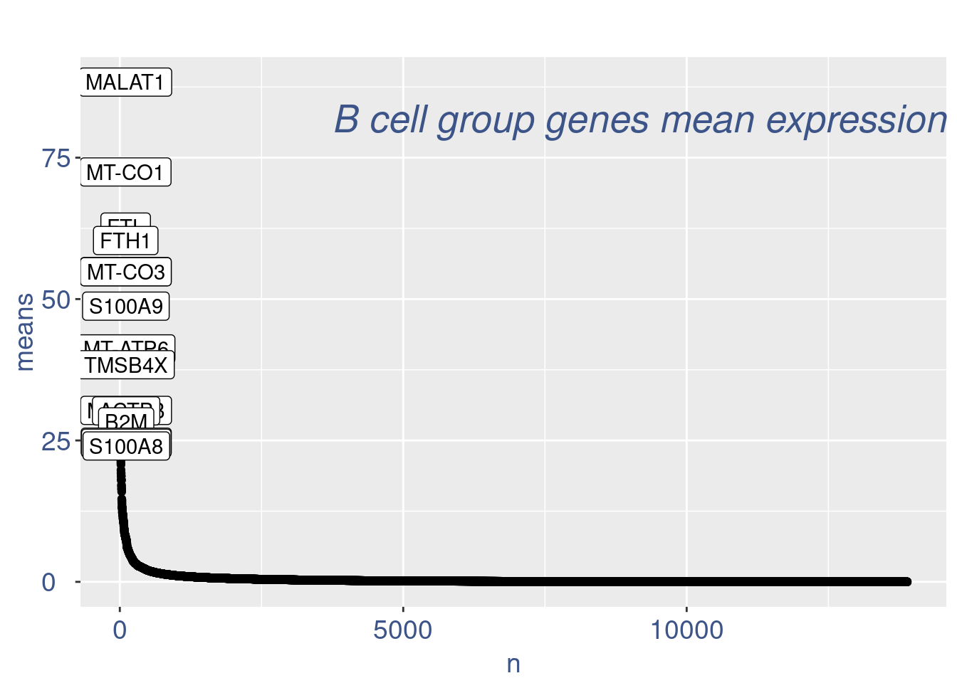
plot(nu)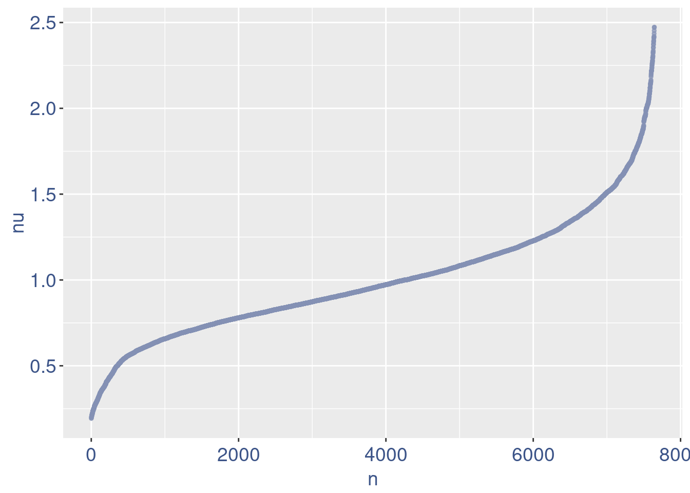
plot(zoomedNu)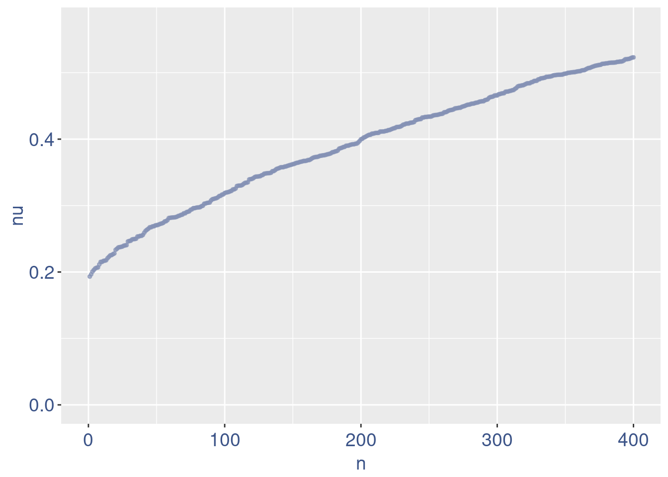
cellSizePlot(aRunObj, condName = "Sample.IDs")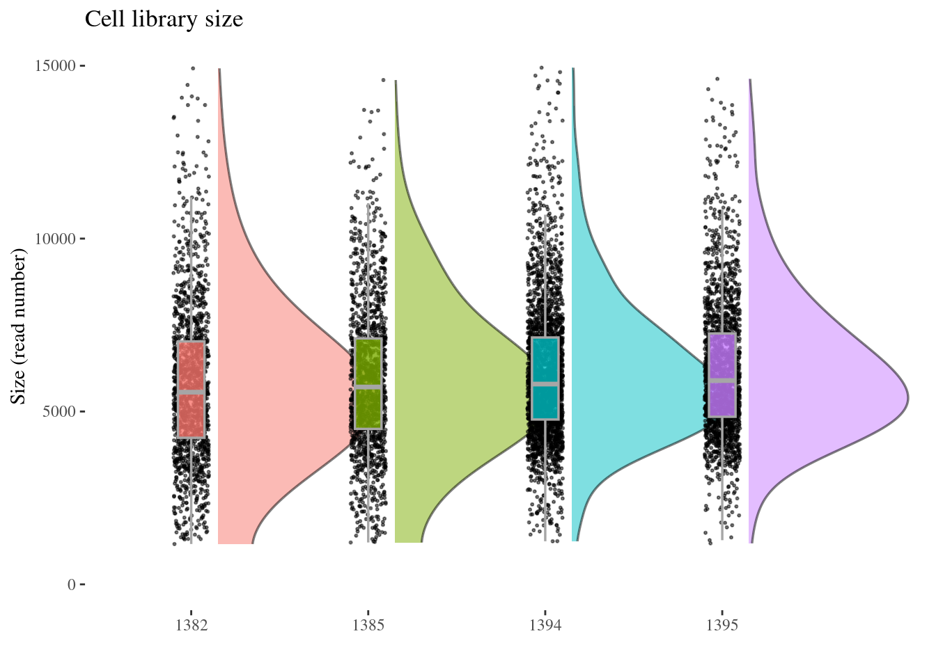
genesSizePlot(aRunObj, condName = "Sample.IDs")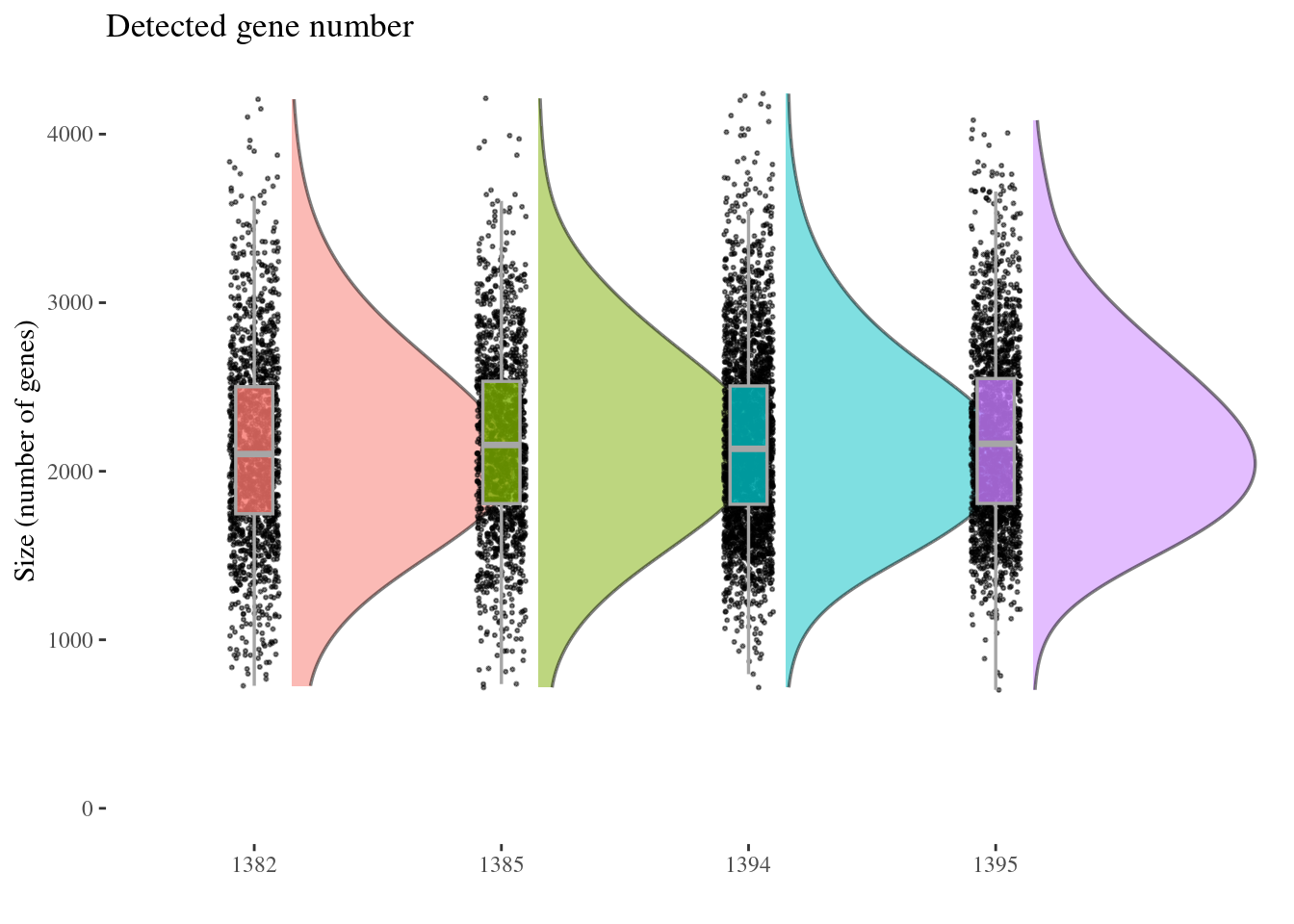
scatterPlot(aRunObj, condName = "Sample.IDs")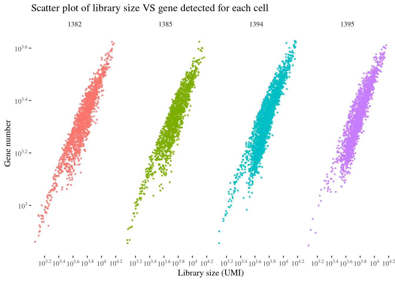
cellSizePlot(aRunObj, condName = "Participant.IDs")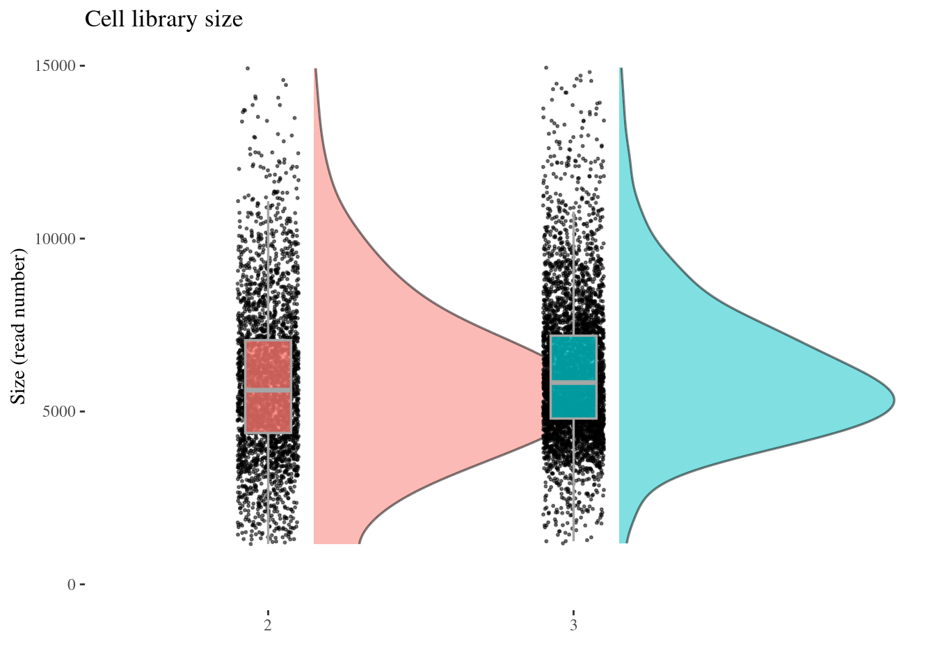
genesSizePlot(aRunObj, condName = "Participant.IDs")
scatterPlot(aRunObj, condName = "Participant.IDs")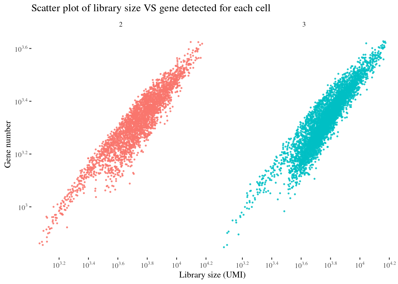
c(mitPerPlot, mitPerDf) %<-%
  mitochondrialPercentagePlot(aRunObj, condName = "Participant.IDs",
                              genePrefix = "^MT-")
mitPerPlot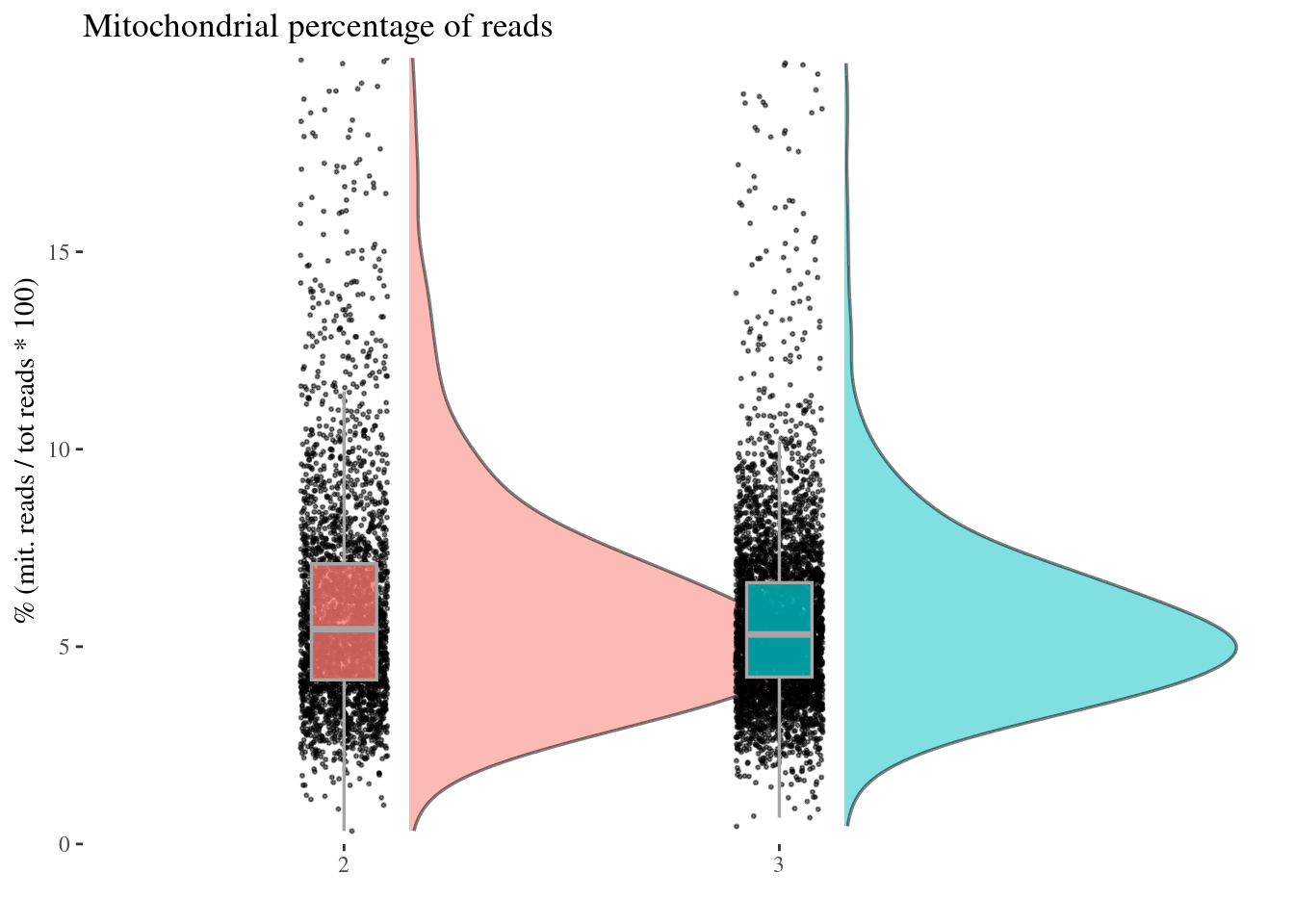
Finalize object and save
aRunObj <- proceedToCoex(aRunObj, calcCoex = TRUE, cores = 1L, saveObj = FALSE)fileNameOut <- paste0(globalCondition, "-Run_", thisRun, "-Cleaned", ".RDS")
saveRDS(aRunObj, file = file.path(inDir, fileNameOut))df <- UDE@data
df$Participant.IDs <- NA
df$Sample.IDs <- NA
df$lane <- NA
df$Participant.IDs <-getCondition(aRunObj,condName = "Participant.IDs")
df$Sample.IDs <- getCondition(aRunObj,condName = "Sample.IDs")
df$lane <-getCondition(aRunObj,condName = "Lane")
df$Sample.IDs <- as.character(df$Sample.IDs)
df$Participant.IDs <- as.character(df$Participant.IDs)
df$lane <- as.character(df$lane)
ggplot(df,aes(x=PC1,y=PC2,color = Participant.IDs)) +geom_point()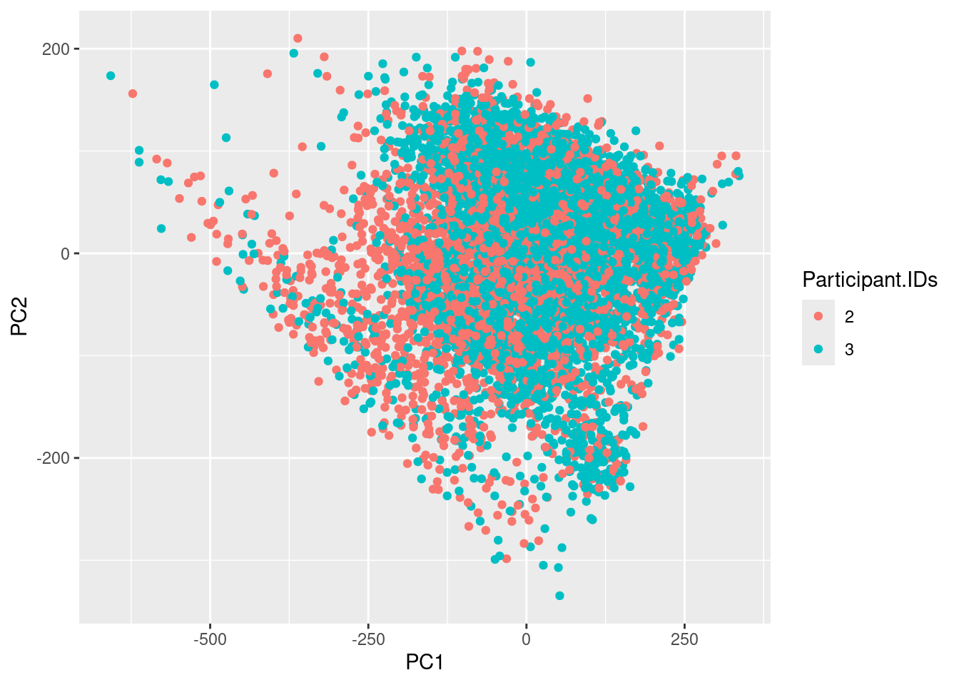
ggplot(df,aes(x=PC1,y=PC2,color = Sample.IDs)) +geom_point()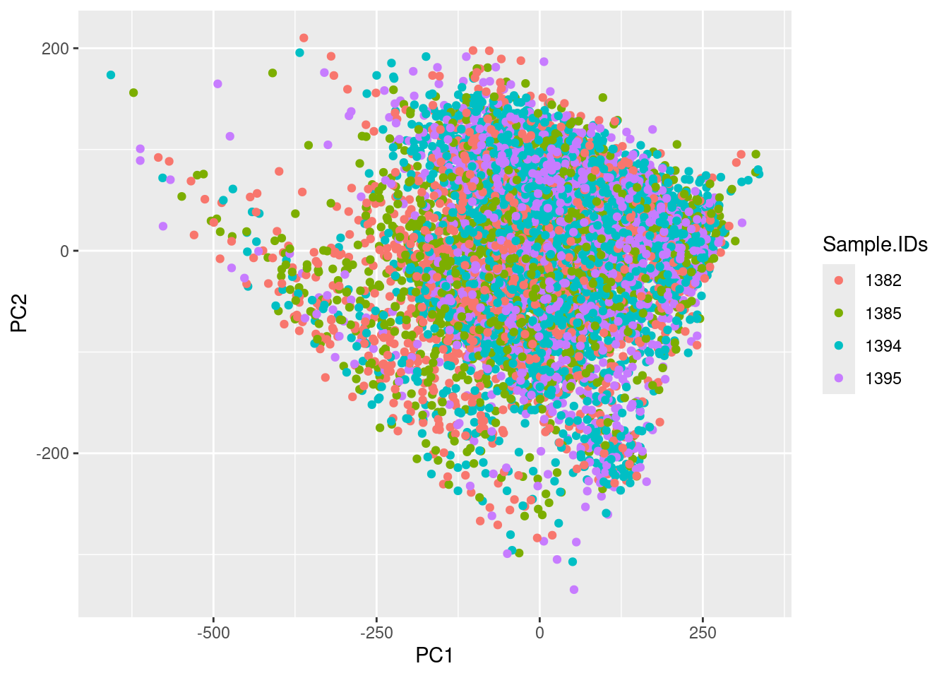
ggplot(df,aes(x=PC1,y=PC2,color = lane)) +geom_point()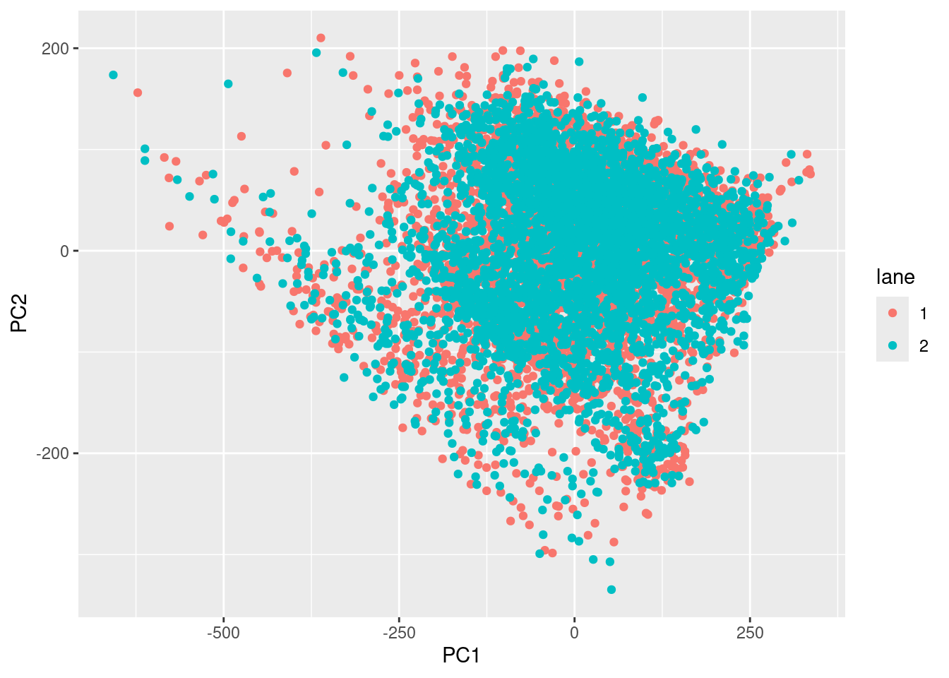
ggplot(df,aes(x=PC1,y=PC3,color = Participant.IDs)) +geom_point()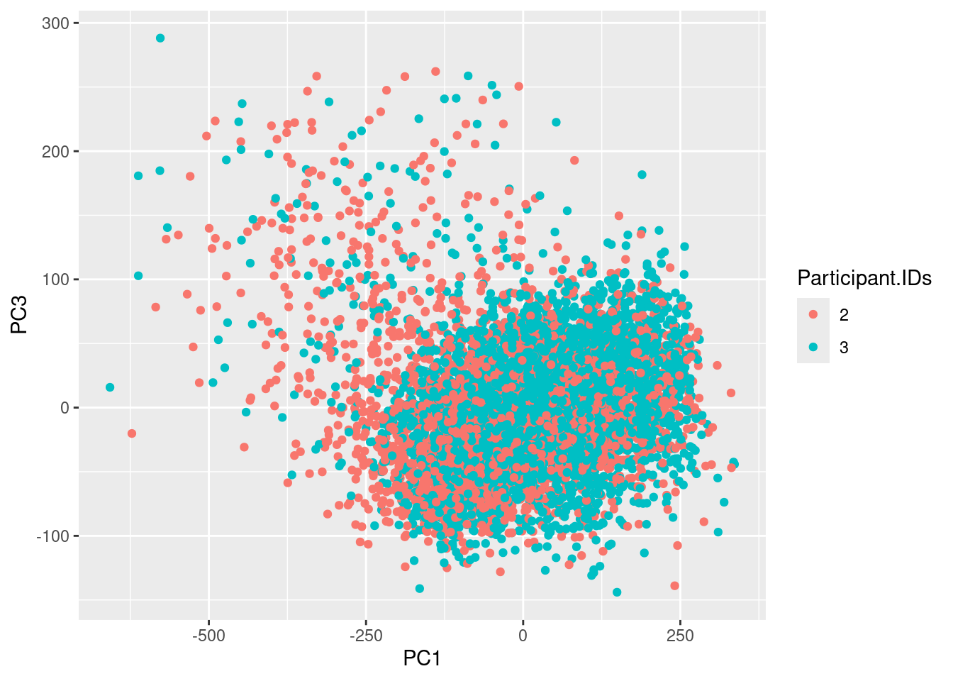
ggplot(df,aes(x=PC1,y=PC3,color = Sample.IDs)) +geom_point()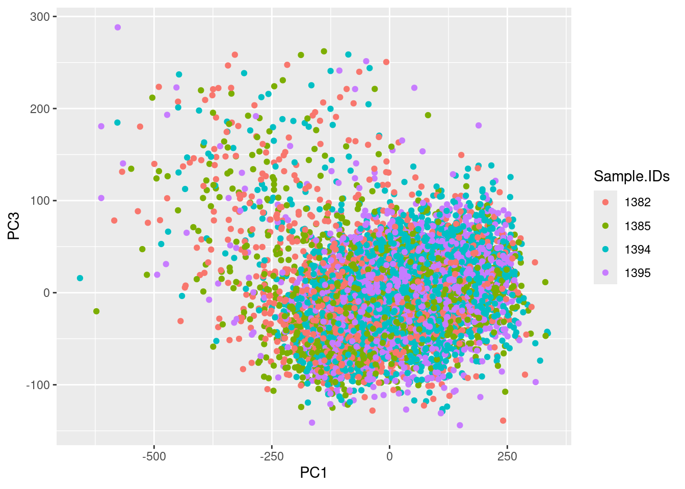
ggplot(df,aes(x=PC1,y=PC3,color = lane)) +geom_point()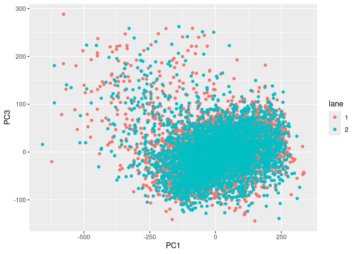
ggplot(df,aes(x=PC1,y=PC4,color = Participant.IDs)) +geom_point()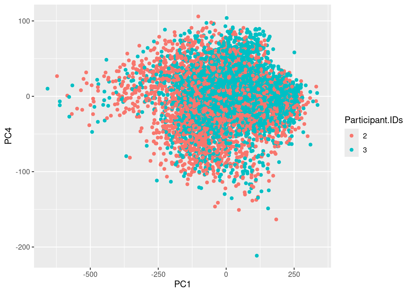
ggplot(df,aes(x=PC1,y=PC4,color = Sample.IDs)) +geom_point()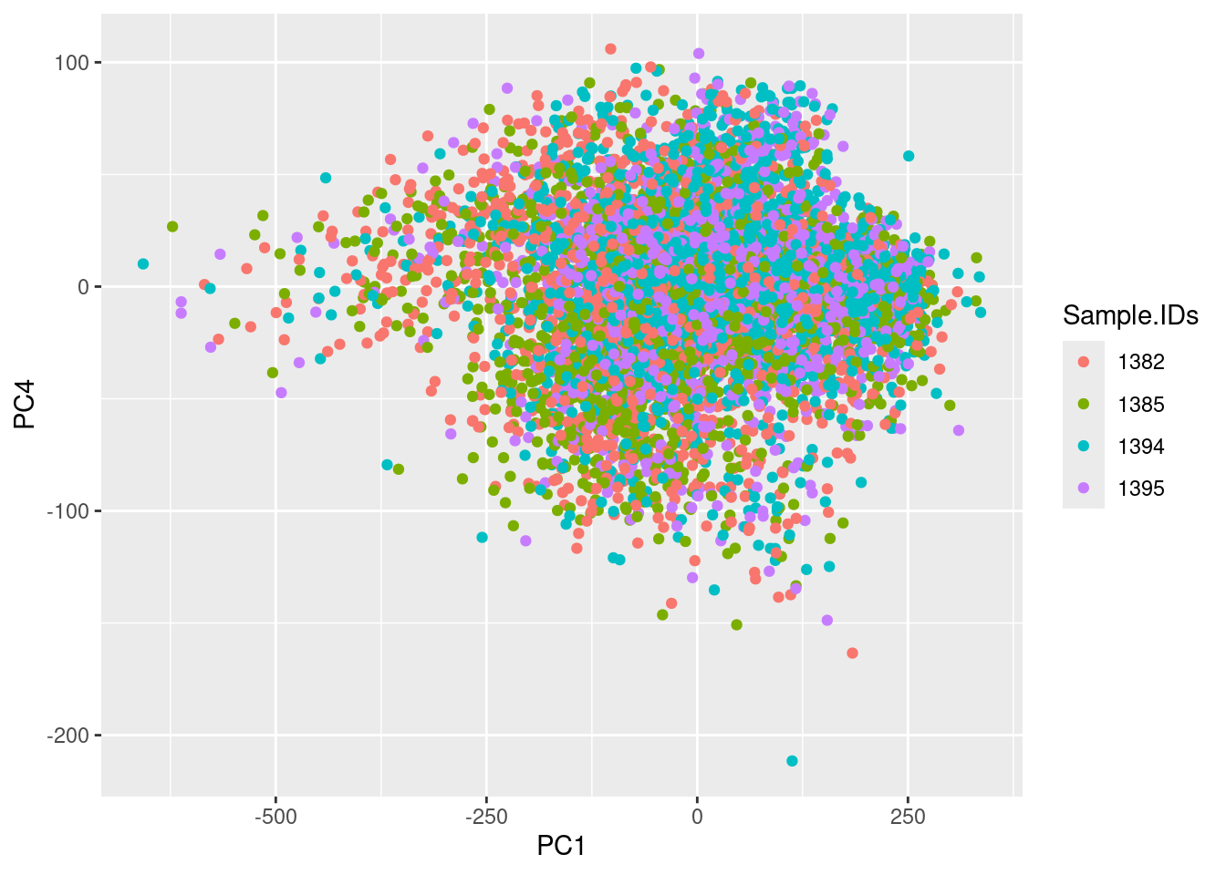
ggplot(df,aes(x=PC1,y=PC4,color = lane)) +geom_point()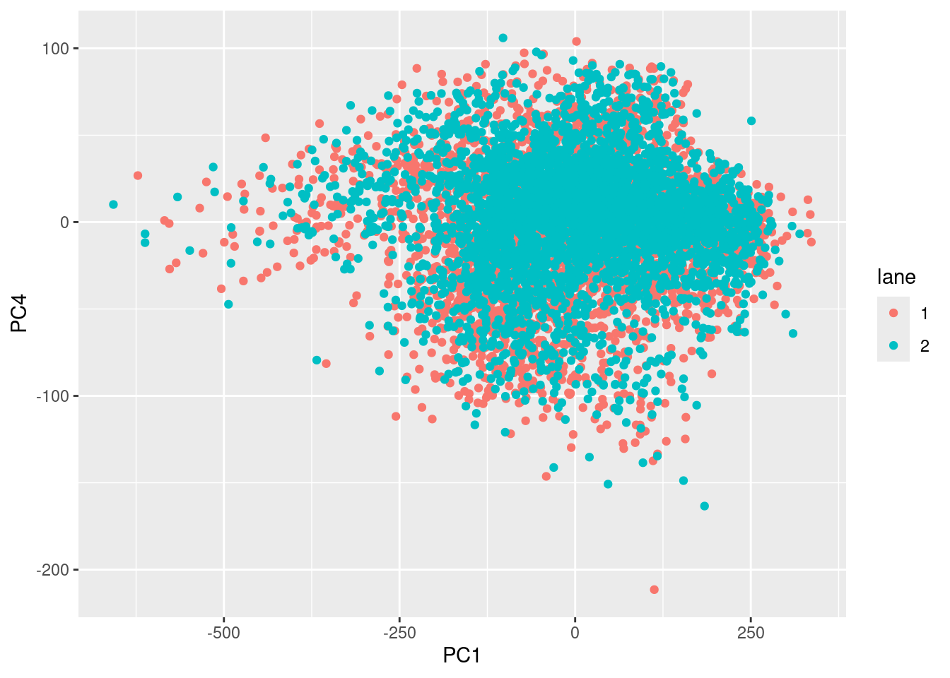
Sys.time()[1] "2026-01-26 11:02:33 CET"sessionInfo()R version 4.5.2 (2025-10-31)
Platform: x86_64-pc-linux-gnu
Running under: Ubuntu 22.04.5 LTS
Matrix products: default
BLAS: /usr/lib/x86_64-linux-gnu/blas/libblas.so.3.10.0
LAPACK: /usr/lib/x86_64-linux-gnu/lapack/liblapack.so.3.10.0 LAPACK version 3.10.0
locale:
[1] LC_CTYPE=C.UTF-8 LC_NUMERIC=C LC_TIME=C.UTF-8
[4] LC_COLLATE=C.UTF-8 LC_MONETARY=C.UTF-8 LC_MESSAGES=C.UTF-8
[7] LC_PAPER=C.UTF-8 LC_NAME=C LC_ADDRESS=C
[10] LC_TELEPHONE=C LC_MEASUREMENT=C.UTF-8 LC_IDENTIFICATION=C
time zone: Europe/Rome
tzcode source: system (glibc)
attached base packages:
[1] stats graphics grDevices utils datasets methods base
other attached packages:
[1] COTAN_2.11.1 Matrix_1.7-4 conflicted_1.2.0 zeallot_0.2.0
[5] ggplot2_4.0.1 assertthat_0.2.1
loaded via a namespace (and not attached):
[1] RcppAnnoy_0.0.22 splines_4.5.2
[3] later_1.4.2 tibble_3.3.0
[5] polyclip_1.10-7 fastDummies_1.7.5
[7] lifecycle_1.0.4 doParallel_1.0.17
[9] globals_0.18.0 lattice_0.22-7
[11] MASS_7.3-65 ggdist_3.3.3
[13] dendextend_1.19.0 magrittr_2.0.4
[15] plotly_4.12.0 rmarkdown_2.29
[17] yaml_2.3.12 httpuv_1.6.16
[19] otel_0.2.0 Seurat_5.4.0
[21] sctransform_0.4.2 spam_2.11-1
[23] sp_2.2-0 spatstat.sparse_3.1-0
[25] reticulate_1.44.1 cowplot_1.2.0
[27] pbapply_1.7-2 RColorBrewer_1.1-3
[29] abind_1.4-8 Rtsne_0.17
[31] GenomicRanges_1.62.1 purrr_1.2.0
[33] BiocGenerics_0.56.0 circlize_0.4.16
[35] GenomeInfoDbData_1.2.14 IRanges_2.44.0
[37] S4Vectors_0.48.0 ggrepel_0.9.6
[39] irlba_2.3.5.1 listenv_0.10.0
[41] spatstat.utils_3.2-1 goftest_1.2-3
[43] RSpectra_0.16-2 spatstat.random_3.4-3
[45] fitdistrplus_1.2-2 parallelly_1.46.0
[47] codetools_0.2-20 DelayedArray_0.36.0
[49] tidyselect_1.2.1 shape_1.4.6.1
[51] UCSC.utils_1.4.0 farver_2.1.2
[53] ScaledMatrix_1.16.0 viridis_0.6.5
[55] matrixStats_1.5.0 stats4_4.5.2
[57] spatstat.explore_3.7-0 Seqinfo_1.0.0
[59] jsonlite_2.0.0 GetoptLong_1.1.0
[61] progressr_0.18.0 ggridges_0.5.6
[63] survival_3.8-3 iterators_1.0.14
[65] foreach_1.5.2 tools_4.5.2
[67] ica_1.0-3 Rcpp_1.1.0
[69] glue_1.8.0 gridExtra_2.3
[71] SparseArray_1.10.8 xfun_0.52
[73] MatrixGenerics_1.22.0 distributional_0.6.0
[75] ggthemes_5.2.0 GenomeInfoDb_1.44.0
[77] dplyr_1.1.4 withr_3.0.2
[79] fastmap_1.2.0 digest_0.6.37
[81] rsvd_1.0.5 parallelDist_0.2.6
[83] R6_2.6.1 mime_0.13
[85] colorspace_2.1-1 scattermore_1.2
[87] tensor_1.5 spatstat.data_3.1-9
[89] tidyr_1.3.1 generics_0.1.3
[91] data.table_1.18.0 httr_1.4.7
[93] htmlwidgets_1.6.4 S4Arrays_1.10.1
[95] uwot_0.2.3 pkgconfig_2.0.3
[97] gtable_0.3.6 ComplexHeatmap_2.26.0
[99] lmtest_0.9-40 S7_0.2.1
[101] SingleCellExperiment_1.32.0 XVector_0.50.0
[103] htmltools_0.5.8.1 dotCall64_1.2
[105] zigg_0.0.2 clue_0.3-66
[107] SeuratObject_5.3.0 scales_1.4.0
[109] Biobase_2.70.0 png_0.1-8
[111] spatstat.univar_3.1-6 knitr_1.50
[113] reshape2_1.4.4 rjson_0.2.23
[115] nlme_3.1-168 proxy_0.4-29
[117] cachem_1.1.0 zoo_1.8-14
[119] GlobalOptions_0.1.2 stringr_1.6.0
[121] KernSmooth_2.23-26 parallel_4.5.2
[123] miniUI_0.1.2 pillar_1.11.1
[125] grid_4.5.2 vctrs_0.7.0
[127] RANN_2.6.2 promises_1.5.0
[129] BiocSingular_1.26.1 beachmat_2.26.0
[131] xtable_1.8-4 cluster_2.1.8.1
[133] evaluate_1.0.5 cli_3.6.5
[135] compiler_4.5.2 rlang_1.1.7
[137] crayon_1.5.3 future.apply_1.20.0
[139] labeling_0.4.3 plyr_1.8.9
[141] stringi_1.8.7 viridisLite_0.4.2
[143] deldir_2.0-4 BiocParallel_1.44.0
[145] lazyeval_0.2.2 spatstat.geom_3.7-0
[147] RcppHNSW_0.6.0 patchwork_1.3.2
[149] future_1.69.0 shiny_1.12.1
[151] SummarizedExperiment_1.38.1 ROCR_1.0-11
[153] Rfast_2.1.5.1 igraph_2.2.1
[155] memoise_2.0.1 RcppParallel_5.1.10