library(COTAN)
library(ComplexHeatmap)
library(circlize)
library(dplyr)
library(Hmisc)
library(Seurat)
library(patchwork)
library(Rfast)
library(parallel)
library(doParallel)
library(HiClimR)
library(stringr)
library(fst)

options(parallelly.fork.enable = TRUE)Gene Correlation Analysis for Mouse Cortex Open Problem
Prologue
dataFile <- "Data/NewDataRevision/Ding_GSE132044_H_PBMC_M_Brain_CleanedDatasets/SplitLoomsAsCOTANObjects/mouse-brain-10XV2_Cortex2_specimen1_cell2-Cleaned.RDS"

name <- str_split(dataFile,pattern = "/",simplify = T)[5]
name <- str_remove(name,pattern = "-Cleaned.RDS")

project = name

setLoggingLevel(1)
outDir <- "CoexData/"
setLoggingFile(paste0(outDir, "Logs/",name,".log"))

obj <- readRDS(dataFile)
file_code = namesource("src/Functions.R")To compare the ability of COTAN to asses the real correlation between genes we define some pools of genes:
- Constitutive genes
- Neural progenitor genes
- Pan neuronal genes
- Some layer marker genes
genesList <- list(
  "NPGs"=
    c("Nes", "Vim", "Sox2", "Sox1", "Notch1", "Hes1", "Hes5", "Pax6"),
  "PNGs"=
    c("Map2", "Tubb3", "Neurod1", "Nefm", "Nefl", "Dcx", "Tbr1"),
  "hk"=
    c("Calm1", "Cox6b1", "Ppia", "Rpl18", "Cox7c", "Erh", "H3f3a",
      "Taf1", "Taf2", "Gapdh", "Actb", "Golph3", "Zfr", "Sub1",
      "Tars", "Amacr"),
  "layers" =
    c("Reln","Lhx5","Cux1","Satb2","Tle1","Mef2c","Rorb","Sox5","Bcl11b","Fezf2","Foxp2","Ntf3","Rasgrf2","Pvrl3", "Cux2","Slc17a6", "Sema3c","Thsd7a", "Sulf2", "Kcnk2","Grik3", "Etv1", "Tle4", "Tmem200a", "Glra2", "Etv1","Htr1f", "Sulf1","Rxfp1", "Syt6")
  # From https://www.science.org/doi/10.1126/science.aam8999
)
COTAN
genesFromListExpressed <- unlist(genesList)[unlist(genesList) %in% getGenes(obj)]
int.genes <-getGenes(obj)
coexMat.big <- getGenesCoex(obj)[genesFromListExpressed,genesFromListExpressed]
coexMat <- getGenesCoex(obj)[c(genesList$NPGs,genesList$hk,genesList$PNGs),c(genesList$NPGs,genesList$hk,genesList$PNGs)]
f1 = colorRamp2(seq(-0.5,0.5, length = 3), c("#DC0000B2", "white","#3C5488B2" ))
split.genes <- base::factor(c(rep("NPGs",length(genesList[["NPGs"]])),
rep("HK",length(genesList[["hk"]])),
rep("PNGs",length(genesList[["PNGs"]]))
),
levels = c("NPGs","HK","PNGs"))
lgd = Legend(col_fun = f1, title = "COTAN coex")
htmp <- Heatmap(as.matrix(coexMat),
#width = ncol(coexMat)*unit(2.5, "mm"),
height = nrow(coexMat)*unit(3, "mm"),
cluster_rows = FALSE,
cluster_columns = FALSE,
col = f1,
row_names_side = "left",
row_names_gp = gpar(fontsize = 11),
column_names_gp = gpar(fontsize = 11),
column_split = split.genes,
row_split = split.genes,
cluster_row_slices = FALSE,
cluster_column_slices = FALSE,
heatmap_legend_param = list(
title = "COTAN coex", at = c(-0.5, 0, 0.5),
direction = "horizontal",
labels = c("-0.5", "0", "0.5")
)
)
draw(htmp, heatmap_legend_side="right")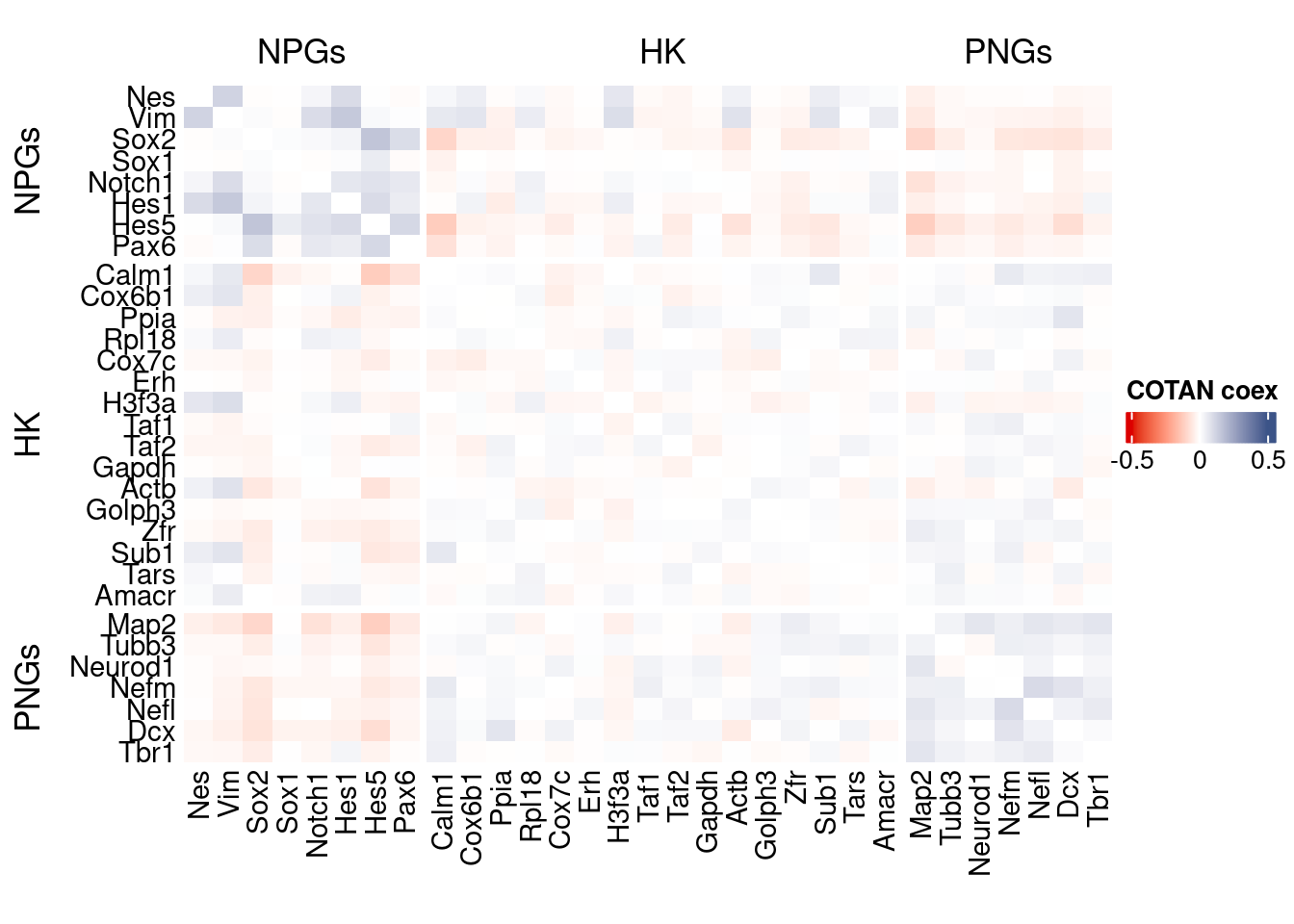
GDI_DF <- calculateGDI(obj)
GDI_DF$geneType <- NA
for (cat in names(genesList)) {
  GDI_DF[rownames(GDI_DF) %in% genesList[[cat]],]$geneType <- cat
}

GDI_DF$GDI_centered <- scale(GDI_DF$GDI,center = T,scale = T)

GDI_DF[genesFromListExpressed,]
sum.raw.norm GDI exp.cells geneType GDI_centered
Nes 3.379037 2.255674 0.4571429 NPGs 2.315313601
Vim 4.681034 2.919354 1.2800000 NPGs 4.233014332
Sox2 6.149767 2.539384 5.4857143 NPGs 3.135092176
Sox1 3.113734 1.107632 0.4342857 NPGs -1.001951237
Notch1 4.461974 1.981517 1.3028571 NPGs 1.523136160
Hes1 5.935441 2.294572 6.0114286 NPGs 2.427708091
Hes5 6.864813 2.726088 7.1771429 NPGs 3.674571519
Pax6 5.402738 2.055585 2.3771429 NPGs 1.737155449
Map2 7.596870 2.583522 34.6971429 PNGs 3.262629249
Tubb3 6.183515 1.501005 9.3942857 PNGs 0.134698949
Neurod1 4.300190 1.783054 2.0800000 PNGs 0.949678059
Nefm 5.581120 1.958701 6.4228571 PNGs 1.457209784
Nefl 6.262705 1.600205 9.4400000 PNGs 0.421338166
Dcx 6.402153 2.030151 12.6628571 PNGs 1.663665101
Tbr1 5.258476 1.603367 4.5942857 PNGs 0.430474312
Calm1 8.361407 2.007616 50.2628571 hk 1.598548962
Cox6b1 6.635892 1.630012 12.5714286 hk 0.507465261
Ppia 5.513003 1.686902 5.9428571 hk 0.671848304
Rpl18 5.255162 1.549301 3.9085714 hk 0.274248941
Cox7c 6.208609 1.355570 9.3714286 hk -0.285536252
Erh 3.048782 1.036642 0.4800000 hk -1.207075994
H3f3a 5.616846 1.703998 4.9371429 hk 0.721247215
Taf1 5.000148 1.312550 3.2228571 hk -0.409840883
Taf2 5.859564 1.465798 7.5885714 hk 0.032967158
Gapdh 4.213034 1.172817 1.2114286 hk -0.813600348
Actb 8.631913 1.959923 45.2571429 hk 1.460741796
Golph3 4.175129 1.247797 1.3257143 hk -0.596944963
Zfr 6.434988 1.650993 13.6685714 hk 0.568090095
Sub1 6.583660 1.660050 13.9200000 hk 0.594259391
Tars 4.852469 1.295711 2.6742857 hk -0.458498501
Amacr 3.999262 1.318422 0.9828571 hk -0.392872684
Reln 4.948763 1.459264 2.6742857 layers 0.014089474
Cux1 6.588607 1.692560 13.5542857 layers 0.688196232
Satb2 5.346668 1.705347 5.3028571 layers 0.725145810
Tle1 5.458904 1.673684 4.8000000 layers 0.633655718
Mef2c 8.432593 3.178532 48.7771429 layers 4.981908321
Rorb 6.886411 1.942459 12.3885714 layers 1.410279524
Sox5 5.283835 1.642217 4.2971429 layers 0.542732024
Bcl11b 6.191476 1.755073 9.2342857 layers 0.868827621
Fezf2 5.775481 1.798057 6.0114286 layers 0.993029350
Foxp2 5.771025 1.483334 5.4857143 layers 0.083638178
Rasgrf2 4.721771 1.435362 2.6285714 layers -0.054974821
Cux2 7.073611 2.242028 17.1885714 layers 2.275881015
Slc17a6 3.754041 1.040186 0.6400000 layers -1.196835677
Sema3c 5.294516 2.299890 2.8571429 layers 2.443074816
Thsd7a 4.717923 1.402977 2.4228571 layers -0.148551248
Sulf2 4.832832 1.280438 2.3085714 layers -0.502628539
Kcnk2 7.049908 2.014681 18.7657143 layers 1.618964490
Grik3 4.402783 1.457270 1.9657143 layers 0.008326194
Etv1 6.107054 1.423063 6.6971429 layers -0.090514216
Tle4 6.299087 1.571417 9.9885714 layers 0.338153563
Tmem200a 3.942860 1.461959 1.3485714 layers 0.021876039
Glra2 4.837674 1.466631 2.7428571 layers 0.035374107
Etv1.1 6.107054 1.423063 6.6971429 layers -0.090514216
Htr1f 5.774912 1.945130 7.4285714 layers 1.417995573
Sulf1 3.560698 1.318445 0.6628571 layers -0.392806371
Rxfp1 4.669295 1.734628 2.2171429 layers 0.809751817
Syt6 4.473121 1.349278 1.7600000 layers -0.303715827GDIPlot(obj,GDIIn = GDI_DF, genes = genesList,GDIThreshold = 1.4)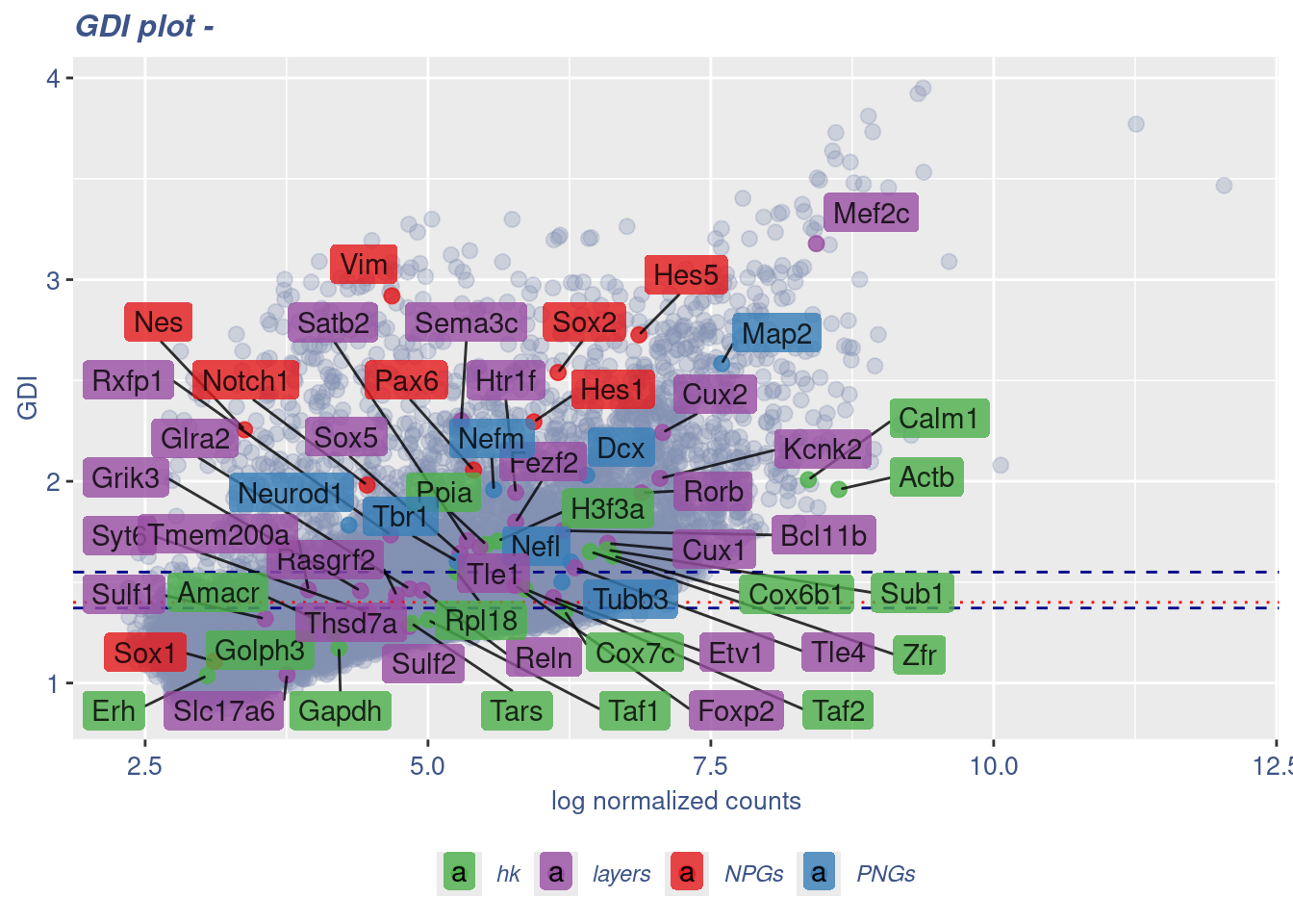
Seurat correlation
srat<- CreateSeuratObject(counts = getRawData(obj),
                          project = project,
                          min.cells = 3,
                          min.features = 200)
srat[["percent.mt"]] <- PercentageFeatureSet(srat, pattern = "^mt-")
srat <- NormalizeData(srat)
srat <- FindVariableFeatures(srat, selection.method = "vst", nfeatures = 2000)

# plot variable features with and without labels
plot1 <- VariableFeaturePlot(srat)

plot1$data$centered_variance <- scale(plot1$data$variance.standardized,
                                      center = T,scale = F)

write.csv(plot1$data,paste0("CoexData/",
                            "Variance_Seurat_genes",
                            getMetadataElement(obj,
                                               datasetTags()[["cond"]]),".csv"))

LabelPoints(plot = plot1, points = c(genesList$NPGs,genesList$PNGs,genesList$layers), repel = TRUE)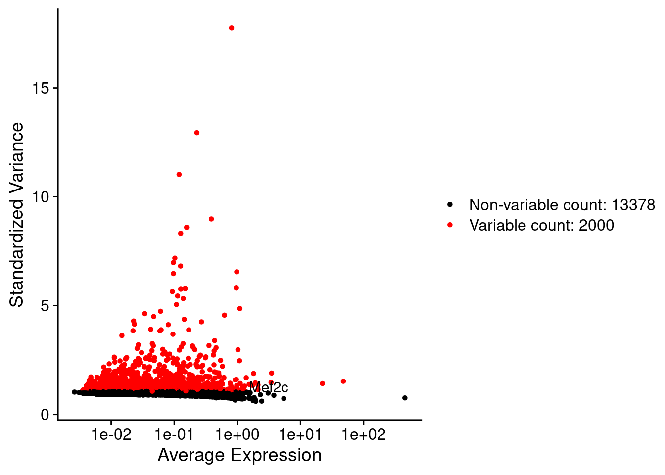
LabelPoints(plot = plot1, points = c(genesList$hk), repel = TRUE)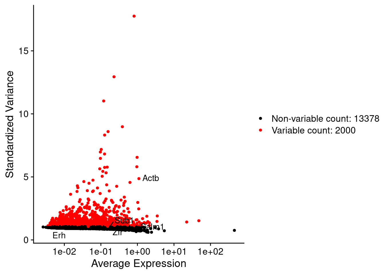
all.genes <- rownames(srat)
srat <- ScaleData(srat, features = all.genes)
seurat.data = GetAssayData(srat[["RNA"]],layer = "data")
corr.pval.list <- correlation_pvalues(data = seurat.data,
genesFromListExpressed,
n.cells = getNumCells(obj))
seurat.data.cor.big <- as.matrix(Matrix::forceSymmetric(corr.pval.list$data.cor, uplo = "U"))
htmp <- correlation_plot(seurat.data.cor.big,
genesList, title="Seurat corr")
p_values.fromSeurat <- corr.pval.list$p_values
seurat.data.cor.big <- corr.pval.list$data.cor
rm(corr.pval.list)
gc() used (Mb) gc trigger (Mb) max used (Mb)
Ncells 10171078 543.2 18206887 972.4 18206887 972.4
Vcells 222385104 1696.7 567605156 4330.5 878334808 6701.2draw(htmp, heatmap_legend_side="right")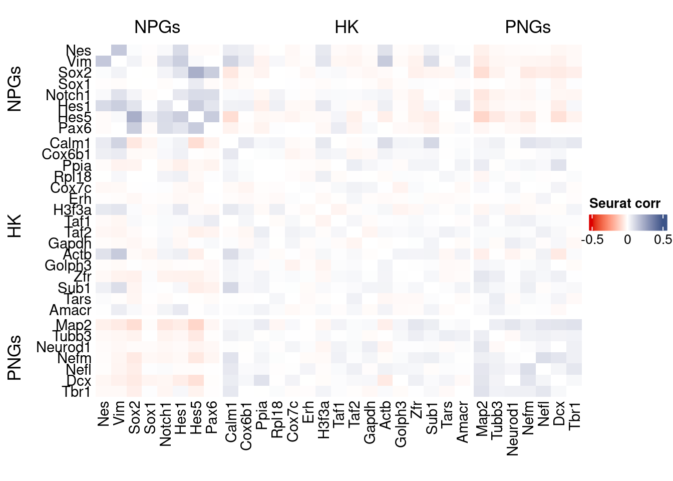
rm(seurat.data.cor.big)
rm(p_values.fromSeurat)
Seurat SC Transform
srat <-  SCTransform(srat,
                     method = "glmGamPoi",
                     vars.to.regress = "percent.mt",
                     verbose = FALSE)

seurat.data <- GetAssayData(srat[["SCT"]],layer = "data")

#Remove genes with all zeros
seurat.data <-seurat.data[rowSums(seurat.data) > 0,]


corr.pval.list <- correlation_pvalues(seurat.data,
                                      genesFromListExpressed,
                                      n.cells = getNumCells(obj))


seurat.data.cor.big <- as.matrix(Matrix::forceSymmetric(corr.pval.list$data.cor, uplo = "U"))

htmp <- correlation_plot(seurat.data.cor.big,
                         genesList, title="Seurat corr SCT")


p_values.fromSeurat <- corr.pval.list$p_values
seurat.data.cor.big <- corr.pval.list$data.cor

rm(corr.pval.list)
gc()
used (Mb) gc trigger (Mb) max used (Mb)
Ncells 10499593 560.8 18206887 972.4 18206887 972.4
Vcells 245389136 1872.2 567605156 4330.5 878334808 6701.2draw(htmp, heatmap_legend_side="right")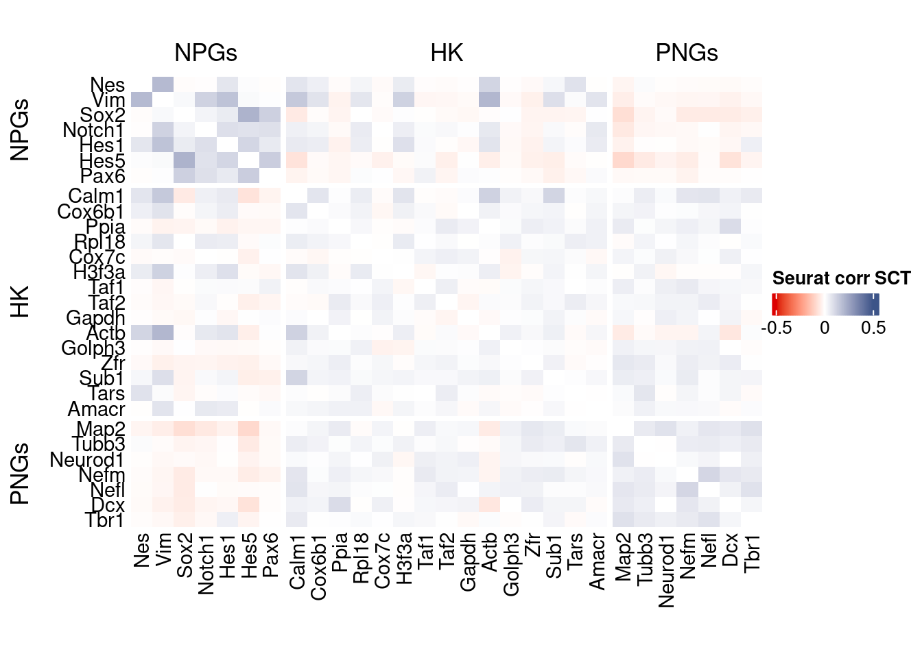
plot1 <- VariableFeaturePlot(srat)

plot1$data$centered_variance <- scale(plot1$data$residual_variance,
center = T,scale = F)write.csv(plot1$data,paste0("CoexData/",
"Variance_SeuratSCT_genes",
getMetadataElement(obj,
datasetTags()[["cond"]]),".csv"))
write_fst(as.data.frame(seurat.data.cor.big),path = paste0("CoexData/SeuratCorrSCT_",file_code,".fst"), compress = 100)
write_fst(as.data.frame(p_values.fromSeurat),path = paste0("CoexData/SeuratPValuesSCT_", file_code,".fst"))
write.csv(as.data.frame(p_values.fromSeurat),paste0("CoexData/SeuratPValuesSCT_", file_code,".csv"))
rm(seurat.data.cor.big)
rm(p_values.fromSeurat)Monocle
library(monocle3)cds <- new_cell_data_set(getRawData(obj),
cell_metadata = getMetadataCells(obj),
gene_metadata = getMetadataGenes(obj)
)
cds <- preprocess_cds(cds, num_dim = 100)
normalized_counts <- normalized_counts(cds)#Remove genes with all zeros
normalized_counts <- normalized_counts[rowSums(normalized_counts) > 0,]
corr.pval.list <- correlation_pvalues(normalized_counts,
genesFromListExpressed,
n.cells = getNumCells(obj))
rm(normalized_counts)
monocle.data.cor.big <- as.matrix(Matrix::forceSymmetric(corr.pval.list$data.cor, uplo = "U"))
htmp <- correlation_plot(data.cor.big = monocle.data.cor.big,
genesList,
title = "Monocle corr")
p_values.from.monocle <- corr.pval.list$p_values
monocle.data.cor.big <- corr.pval.list$data.cor
rm(corr.pval.list)
gc() used (Mb) gc trigger (Mb) max used (Mb)
Ncells 10685853 570.7 18206887 972.4 18206887 972.4
Vcells 247725848 1890.0 567605156 4330.5 878334808 6701.2draw(htmp, heatmap_legend_side="right")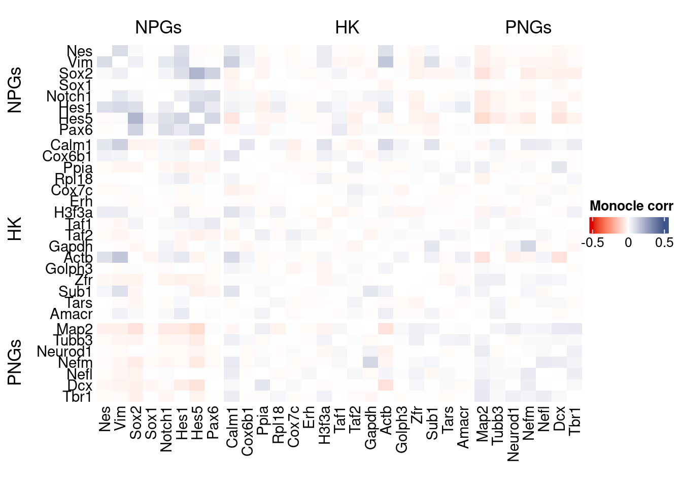
ScanPy
library(reticulate)

dirOutScP <- paste0("CoexData/ScanPy/")
if (!dir.exists(dirOutScP)) {
  dir.create(dirOutScP)
}
if(Sys.info()[["sysname"]] == "Windows"){

  use_python("C:/Users/Silvia/miniconda3/envs/r-scanpy/python.exe", required = TRUE)
  #Sys.setenv(RETICULATE_PYTHON = "C:/Users/Silvia/AppData/Local/Python/pythoncore-3.14-64/python.exe" )
}else{
  Sys.setenv(RETICULATE_PYTHON = "../../../bin/python3")
}

  py <- import("sys")

  source_python("src/scanpyGenesExpression.py")
  scanpyFDR(getRawData(obj),
                  getMetadataCells(obj),
                  getMetadataGenes(obj),
                   "mt",
                   dirOutScP,
                   file_code,
            int.genes)
inizio
open pdfnormalized_counts <- read.csv(paste0(dirOutScP,
file_code,"_Scanpy_expression_all_genes.gz"),header = T,row.names = 1)
normalized_counts <- t(normalized_counts)#Remove genes with all zeros
normalized_counts <-normalized_counts[rowSums(normalized_counts) > 0,]
corr.pval.list <- correlation_pvalues(normalized_counts,
genesFromListExpressed,
n.cells = getNumCells(obj))
ScanPy.data.cor.big <- as.matrix(Matrix::forceSymmetric(corr.pval.list$data.cor, uplo = "U"))
htmp <- correlation_plot(data.cor.big = ScanPy.data.cor.big,
genesList,
title = "ScanPy corr")
p_values.from.ScanPy <- corr.pval.list$p_values
ScanPy.data.cor.big <- corr.pval.list$data.cor
rm(corr.pval.list)
gc() used (Mb) gc trigger (Mb) max used (Mb)
Ncells 10706858 571.9 18206887 972.4 18206887 972.4
Vcells 315072036 2403.9 567605156 4330.5 878334808 6701.2draw(htmp, heatmap_legend_side="right")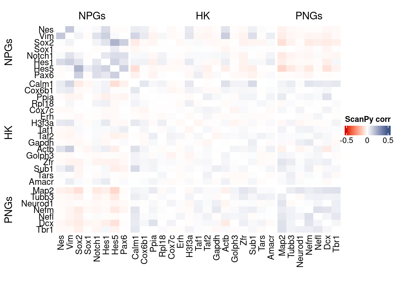
Cs-Core
library(CSCORE)Convert to Seurat obj
sceObj <- convertToSingleCellExperiment(obj)

# Correct: assay=NULL (or omit), data=NULL (since no logcounts)
seuratObj <- as.Seurat(
  x       = sceObj,
  counts  = "counts",
  data    = NULL,
  assay   = NULL,      # IMPORTANT: do NOT set to "RNA" here
  project = "COTAN"
)

# as.Seurat(SCE) creates assay "originalexp" by default; rename it to RNA
seuratObj <- RenameAssays(seuratObj, originalexp = "RNA", verbose = FALSE)
DefaultAssay(seuratObj) <- "RNA"

# Optional: keep COTAN payload
seuratObj@misc$COTAN <- S4Vectors::metadata(sceObj)
Extract CS_CORE corr matrix
#seuratObj@assays$RNA@counts <- ceiling(seuratObj@assays$RNA@counts)
csCoreRes <- CSCORE(seuratObj, genes = genesFromListExpressed)
[INFO] IRLS converged after 3 iterations.
[INFO] Starting WLS for covariance at Fri Jan 23 11:03:54 2026
[INFO] 7 among 58 genes have invalid variance estimates. Their co-expressions with other genes were set to 0.
[INFO] 0.8469% co-expression estimates were greater than 1 and were set to 1.
[INFO] 0.2420% co-expression estimates were smaller than -1 and were set to -1.
[INFO] Finished WLS. Elapsed time: 0.1160 seconds.mat <- as.matrix(csCoreRes$est)
diag(mat) <- 0
split.genes <- base::factor(c(rep("NPGs",sum(genesList[["NPGs"]] %in% genesFromListExpressed)),
rep("HK",sum(genesList[["hk"]] %in% genesFromListExpressed)),
rep("PNGs",sum(genesList[["PNGs"]] %in% genesFromListExpressed))
),
levels = c("NPGs","HK","PNGs"))
f1 = colorRamp2(seq(-0.5,0.5, length = 3), c("#DC0000B2", "white","#3C5488B2" ))
htmp <- Heatmap(as.matrix(mat[c(genesList$NPGs,genesList$hk,genesList$PNGs),c(genesList$NPGs,genesList$hk,genesList$PNGs)]),
#width = ncol(coexMat)*unit(2.5, "mm"),
height = nrow(mat)*unit(3, "mm"),
cluster_rows = FALSE,
cluster_columns = FALSE,
col = f1,
row_names_side = "left",
row_names_gp = gpar(fontsize = 11),
column_names_gp = gpar(fontsize = 11),
column_split = split.genes,
row_split = split.genes,
cluster_row_slices = FALSE,
cluster_column_slices = FALSE,
heatmap_legend_param = list(
title = "CS-CORE", at = c(-0.5, 0, 0.5),
direction = "horizontal",
labels = c("-0.5", "0", "0.5")
)
)
draw(htmp, heatmap_legend_side="right")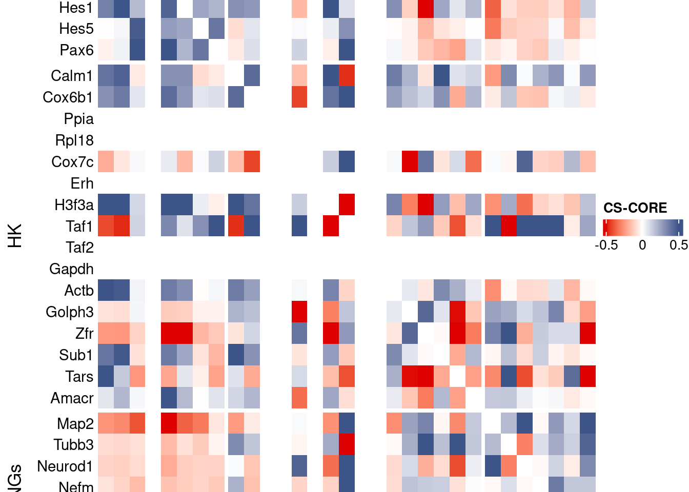
Save CS_CORE matrix
write_fst(as.data.frame(csCoreRes$est), path = paste0("CoexData/CS_CORECorr_", file_code,".fst"),compress = 100)
write_fst(as.data.frame(csCoreRes$p_value), path = paste0("CoexData/CS_COREPValues_", file_code,".fst"),compress = 100)
write.csv(as.data.frame(csCoreRes$p_value), paste0("CoexData/CS_COREPValues_", file_code,".csv"))
Baseline: Spearman on UMI counts
corr.pval.list <- correlation_pvaluesSpearman(data = getRawData(obj),
                                      genesFromListExpressed,
                                      n.cells = getNumCells(obj))

data.cor.big <- as.matrix(Matrix::forceSymmetric(corr.pval.list$data.cor, uplo = "U"))

htmp <- correlation_plot(data.cor.big,
                         genesList, title="UMI baseline S. corr")


p_values.fromSp.C <- corr.pval.list$p_values
data.cor.bigSp.C <- corr.pval.list$data.cor

rm(corr.pval.list)
gc()
used (Mb) gc trigger (Mb) max used (Mb)
Ncells 10715538 572.3 18206887 972.4 18206887 972.4
Vcells 315757239 2409.1 567605156 4330.5 878334808 6701.2draw(htmp, heatmap_legend_side="right")
write.csv(as.data.frame(p_values.fromSp.C), paste0("CoexData/BaselineUMISpCorrPValues_", file_code,".csv"))Baseline: Pearson on binarized counts
corr.pval.list <- correlation_pvalues(data = getZeroOneProj(obj),
                                      genesFromListExpressed,
                                      n.cells = getNumCells(obj))

data.cor.big <- as.matrix(Matrix::forceSymmetric(corr.pval.list$data.cor, uplo = "U"))

htmp <- correlation_plot(data.cor.big,
                         genesList, title="Zero-one P. corr")


p_values.fromSp.C <- corr.pval.list$p_values
data.cor.bigSp.C <- corr.pval.list$data.cor

rm(corr.pval.list)
gc()
used (Mb) gc trigger (Mb) max used (Mb)
Ncells 10715671 572.3 18206887 972.4 18206887 972.4
Vcells 315757506 2409.1 567605156 4330.5 878334808 6701.2draw(htmp, heatmap_legend_side="right")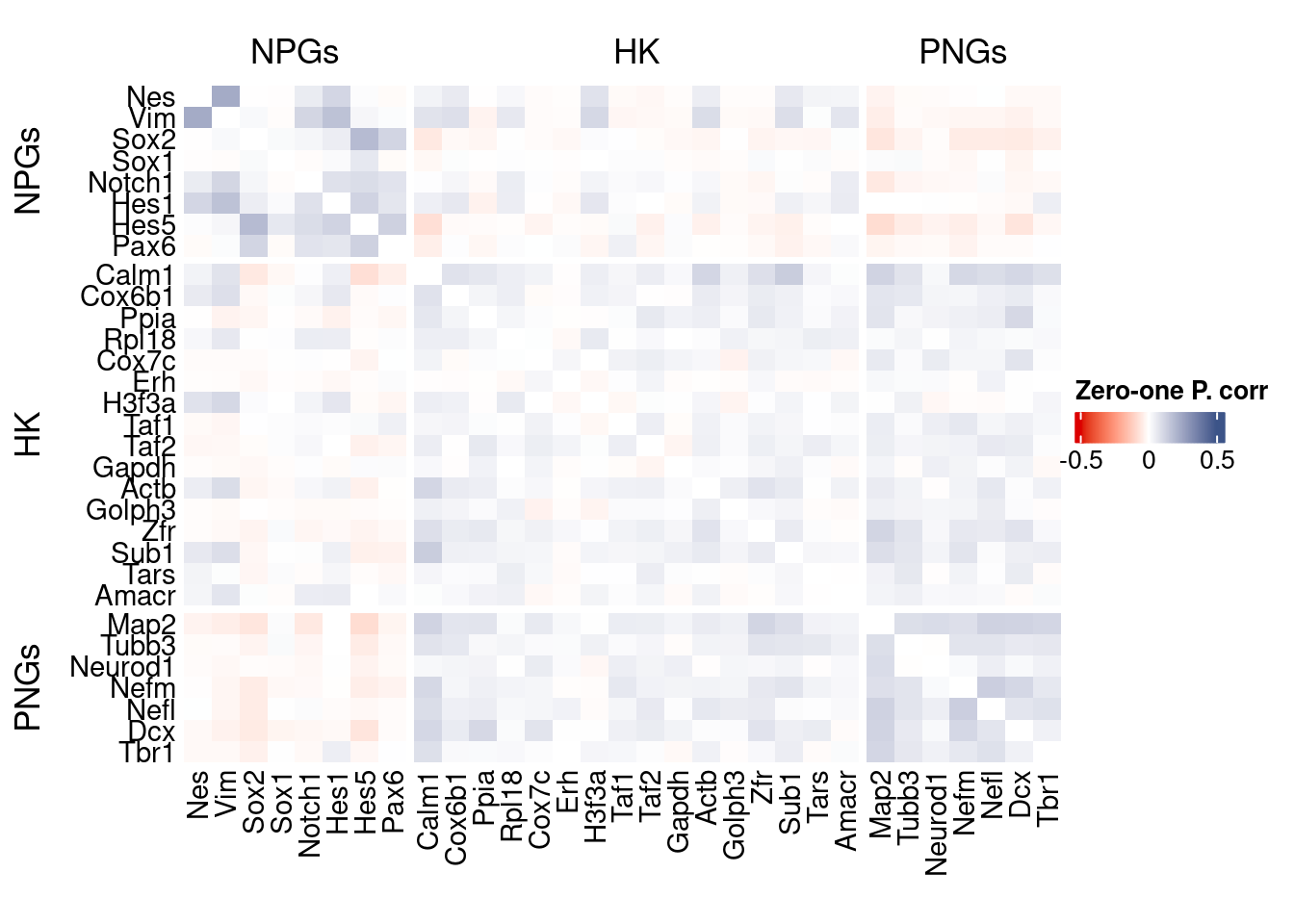
write.csv(as.data.frame(p_values.fromSp.C), paste0("CoexData/ZeroOnePCorrPValues_", file_code,".csv"))Sys.time()[1] "2026-01-23 11:04:00 CET"sessionInfo()R version 4.5.2 (2025-10-31)
Platform: x86_64-pc-linux-gnu
Running under: Ubuntu 22.04.5 LTS
Matrix products: default
BLAS: /usr/lib/x86_64-linux-gnu/blas/libblas.so.3.10.0
LAPACK: /usr/lib/x86_64-linux-gnu/lapack/liblapack.so.3.10.0 LAPACK version 3.10.0
locale:
[1] LC_CTYPE=C.UTF-8 LC_NUMERIC=C LC_TIME=C.UTF-8
[4] LC_COLLATE=C.UTF-8 LC_MONETARY=C.UTF-8 LC_MESSAGES=C.UTF-8
[7] LC_PAPER=C.UTF-8 LC_NAME=C LC_ADDRESS=C
[10] LC_TELEPHONE=C LC_MEASUREMENT=C.UTF-8 LC_IDENTIFICATION=C
time zone: Europe/Rome
tzcode source: system (glibc)
attached base packages:
[1] stats4 parallel grid stats graphics grDevices utils
[8] datasets methods base
other attached packages:
[1] CSCORE_1.0.2 reticulate_1.44.1
[3] monocle3_1.3.7 SingleCellExperiment_1.32.0
[5] SummarizedExperiment_1.38.1 GenomicRanges_1.62.1
[7] Seqinfo_1.0.0 IRanges_2.44.0
[9] S4Vectors_0.48.0 MatrixGenerics_1.22.0
[11] matrixStats_1.5.0 Biobase_2.70.0
[13] BiocGenerics_0.56.0 generics_0.1.3
[15] fstcore_0.10.0 fst_0.9.8
[17] stringr_1.6.0 HiClimR_2.2.1
[19] doParallel_1.0.17 iterators_1.0.14
[21] foreach_1.5.2 Rfast_2.1.5.1
[23] RcppParallel_5.1.10 zigg_0.0.2
[25] Rcpp_1.1.0 patchwork_1.3.2
[27] Seurat_5.4.0 SeuratObject_5.3.0
[29] sp_2.2-0 Hmisc_5.2-3
[31] dplyr_1.1.4 circlize_0.4.16
[33] ComplexHeatmap_2.26.0 COTAN_2.11.1
loaded via a namespace (and not attached):
[1] RcppAnnoy_0.0.22 splines_4.5.2
[3] later_1.4.2 tibble_3.3.0
[5] polyclip_1.10-7 rpart_4.1.24
[7] fastDummies_1.7.5 lifecycle_1.0.4
[9] Rdpack_2.6.4 globals_0.18.0
[11] lattice_0.22-7 MASS_7.3-65
[13] backports_1.5.0 ggdist_3.3.3
[15] dendextend_1.19.0 magrittr_2.0.4
[17] plotly_4.11.0 rmarkdown_2.29
[19] yaml_2.3.10 httpuv_1.6.16
[21] otel_0.2.0 glmGamPoi_1.20.0
[23] sctransform_0.4.2 spam_2.11-1
[25] spatstat.sparse_3.1-0 minqa_1.2.8
[27] cowplot_1.2.0 pbapply_1.7-2
[29] RColorBrewer_1.1-3 abind_1.4-8
[31] Rtsne_0.17 purrr_1.2.0
[33] nnet_7.3-20 GenomeInfoDbData_1.2.14
[35] ggrepel_0.9.6 irlba_2.3.5.1
[37] listenv_0.10.0 spatstat.utils_3.2-1
[39] goftest_1.2-3 RSpectra_0.16-2
[41] spatstat.random_3.4-3 fitdistrplus_1.2-2
[43] parallelly_1.46.0 DelayedMatrixStats_1.30.0
[45] ncdf4_1.24 codetools_0.2-20
[47] DelayedArray_0.36.0 tidyselect_1.2.1
[49] shape_1.4.6.1 UCSC.utils_1.4.0
[51] farver_2.1.2 lme4_1.1-37
[53] ScaledMatrix_1.16.0 viridis_0.6.5
[55] base64enc_0.1-3 spatstat.explore_3.6-0
[57] jsonlite_2.0.0 GetoptLong_1.1.0
[59] Formula_1.2-5 progressr_0.18.0
[61] ggridges_0.5.6 survival_3.8-3
[63] tools_4.5.2 ica_1.0-3
[65] glue_1.8.0 gridExtra_2.3
[67] SparseArray_1.10.8 xfun_0.52
[69] distributional_0.6.0 ggthemes_5.2.0
[71] GenomeInfoDb_1.44.0 withr_3.0.2
[73] fastmap_1.2.0 boot_1.3-32
[75] digest_0.6.37 rsvd_1.0.5
[77] parallelDist_0.2.6 R6_2.6.1
[79] mime_0.13 colorspace_2.1-1
[81] Cairo_1.7-0 scattermore_1.2
[83] tensor_1.5 spatstat.data_3.1-9
[85] tidyr_1.3.1 data.table_1.18.0
[87] httr_1.4.7 htmlwidgets_1.6.4
[89] S4Arrays_1.10.1 uwot_0.2.3
[91] pkgconfig_2.0.3 gtable_0.3.6
[93] lmtest_0.9-40 S7_0.2.1
[95] XVector_0.50.0 htmltools_0.5.8.1
[97] dotCall64_1.2 clue_0.3-66
[99] scales_1.4.0 png_0.1-8
[101] reformulas_0.4.1 spatstat.univar_3.1-6
[103] rstudioapi_0.18.0 knitr_1.50
[105] reshape2_1.4.4 rjson_0.2.23
[107] nloptr_2.2.1 checkmate_2.3.2
[109] nlme_3.1-168 proxy_0.4-29
[111] zoo_1.8-14 GlobalOptions_0.1.2
[113] KernSmooth_2.23-26 miniUI_0.1.2
[115] foreign_0.8-90 pillar_1.11.1
[117] vctrs_0.7.0 RANN_2.6.2
[119] promises_1.5.0 BiocSingular_1.26.1
[121] beachmat_2.26.0 xtable_1.8-4
[123] cluster_2.1.8.1 htmlTable_2.4.3
[125] evaluate_1.0.5 magick_2.9.0
[127] zeallot_0.2.0 cli_3.6.5
[129] compiler_4.5.2 rlang_1.1.7
[131] crayon_1.5.3 future.apply_1.20.0
[133] labeling_0.4.3 plyr_1.8.9
[135] stringi_1.8.7 viridisLite_0.4.2
[137] deldir_2.0-4 BiocParallel_1.44.0
[139] assertthat_0.2.1 lazyeval_0.2.2
[141] spatstat.geom_3.6-1 Matrix_1.7-4
[143] RcppHNSW_0.6.0 sparseMatrixStats_1.20.0
[145] future_1.69.0 ggplot2_4.0.1
[147] shiny_1.12.1 rbibutils_2.3
[149] ROCR_1.0-11 igraph_2.2.1