library(COTAN)
library(ComplexHeatmap)
library(circlize)
library(dplyr)
library(Hmisc)
library(Seurat)
library(patchwork)
library(Rfast)
library(parallel)
library(doParallel)
library(HiClimR)
library(stringr)
library(fst)

options(parallelly.fork.enable = TRUE)Gene Correlation Analysis for Mouse Cortex Open Problem
Prologue
dataFile <- "Data/NewDataRevision/Ding_GSE132044_H_PBMC_M_Brain_CleanedDatasets/SplitLoomsAsCOTANObjects/mouse-brain-SS2_Cortex1_specimen1_cell1-Cleaned.RDS"


name <- str_split(dataFile,pattern = "/",simplify = T)[5]
name <- str_remove(name,pattern = "-Cleaned.RDS")

project = name

setLoggingLevel(1)
outDir <- "CoexData/"
setLoggingFile(paste0(outDir, "Logs/",name,".log"))

obj <- readRDS(dataFile)
file_code = namesource("src/Functions.R")To compare the ability of COTAN to asses the real correlation between genes we define some pools of genes:
- Constitutive genes
- Neural progenitor genes
- Pan neuronal genes
- Some layer marker genes
genesList <- list(
  "NPGs"=
    c("Nes", "Vim", "Sox2", "Sox1", "Notch1", "Hes1", "Hes5", "Pax6"),
  "PNGs"=
    c("Map2", "Tubb3", "Neurod1", "Nefm", "Nefl", "Dcx", "Tbr1"),
  "hk"=
    c("Calm1", "Cox6b1", "Ppia", "Rpl18", "Cox7c", "Erh", "H3f3a",
      "Taf1", "Taf2", "Gapdh", "Actb", "Golph3", "Zfr", "Sub1",
      "Tars", "Amacr"),
  "layers" =
    c("Reln","Lhx5","Cux1","Satb2","Tle1","Mef2c","Rorb","Sox5","Bcl11b","Fezf2","Foxp2","Ntf3","Rasgrf2","Pvrl3", "Cux2","Slc17a6", "Sema3c","Thsd7a", "Sulf2", "Kcnk2","Grik3", "Etv1", "Tle4", "Tmem200a", "Glra2", "Etv1","Htr1f", "Sulf1","Rxfp1", "Syt6")
  # From https://www.science.org/doi/10.1126/science.aam8999
)
COTAN
genesFromListExpressed <- unlist(genesList)[unlist(genesList) %in% getGenes(obj)]
int.genes <-getGenes(obj)
coexMat.big <- getGenesCoex(obj)[genesFromListExpressed,genesFromListExpressed]
coexMat <- coexMat.big[rownames(coexMat.big) %in% c(genesList$NPGs,genesList$hk,genesList$PNGs),
colnames(coexMat.big) %in% c(genesList$NPGs,genesList$hk,genesList$PNGs)]
f1 = colorRamp2(seq(-0.5,0.5, length = 3), c("#DC0000B2", "white","#3C5488B2" ))
split.genes <- base::factor(c(rep("NPGs",sum(genesList[["NPGs"]] %in% getGenes(obj))),
rep("HK",sum(genesList[["hk"]] %in% getGenes(obj))),
rep("PNGs",sum(genesList[["PNGs"]] %in% getGenes(obj)))
),
levels = c("NPGs","HK","PNGs"))
lgd = Legend(col_fun = f1, title = "COTAN coex")
htmp <- Heatmap(as.matrix(coexMat),
#width = ncol(coexMat)*unit(2.5, "mm"),
height = nrow(coexMat)*unit(3, "mm"),
cluster_rows = FALSE,
cluster_columns = FALSE,
col = f1,
row_names_side = "left",
row_names_gp = gpar(fontsize = 11),
column_names_gp = gpar(fontsize = 11),
column_split = split.genes,
row_split = split.genes,
cluster_row_slices = FALSE,
cluster_column_slices = FALSE,
heatmap_legend_param = list(
title = "COTAN coex", at = c(-0.5, 0, 0.5),
direction = "horizontal",
labels = c("-0.5", "0", "0.5")
)
)
draw(htmp, heatmap_legend_side="right")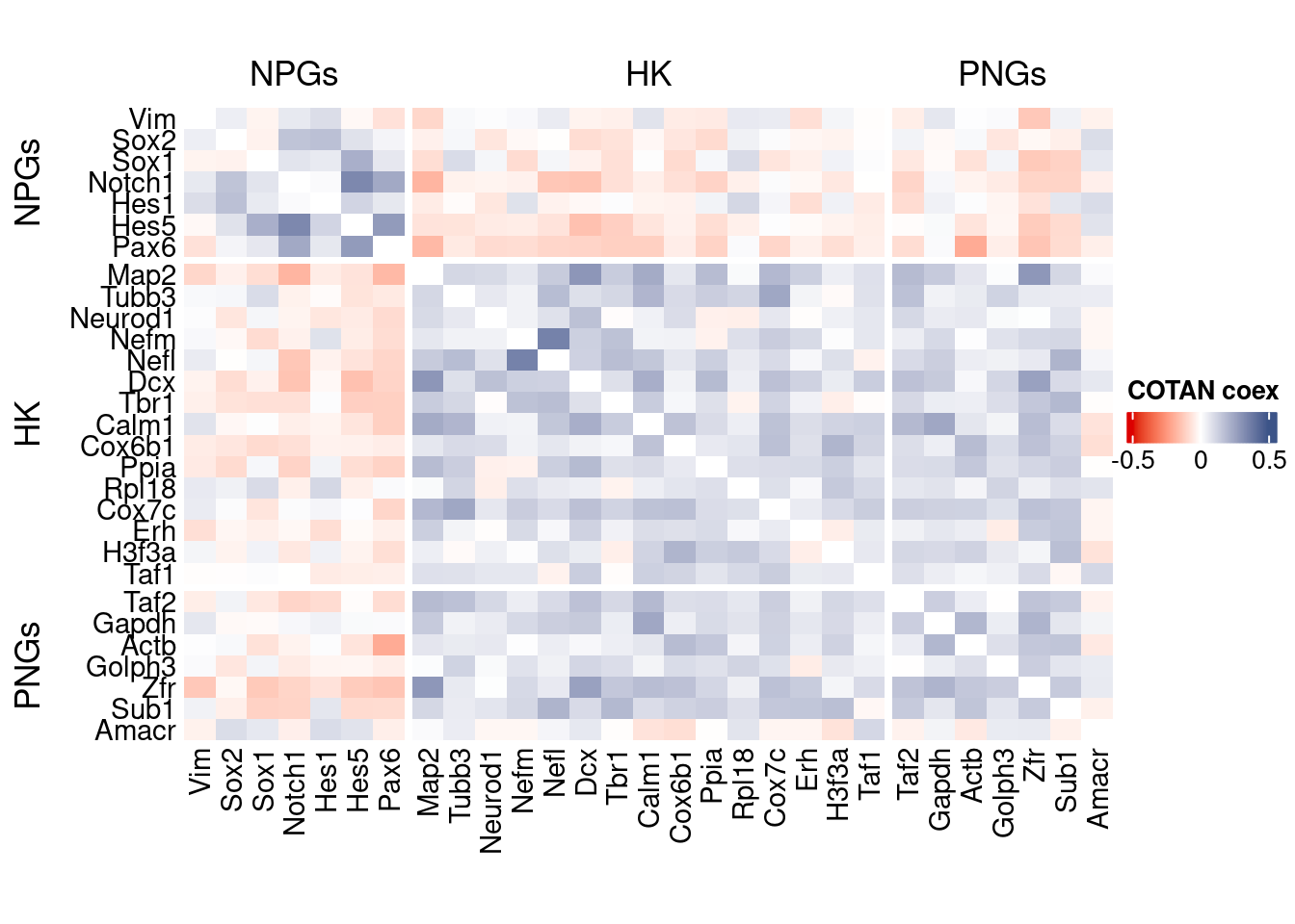
GDI_DF <- calculateGDI(obj)
GDI_DF$geneType <- NA
for (cat in names(genesList)) {
  GDI_DF[rownames(GDI_DF) %in% genesList[[cat]],]$geneType <- cat
}

GDI_DF$GDI_centered <- scale(GDI_DF$GDI,center = T,scale = T)

GDI_DF[genesFromListExpressed,]
sum.raw.norm GDI exp.cells geneType GDI_centered
Vim 7.890070 1.625653 3.767123 NPGs -0.33619863
Sox2 6.590674 1.766255 4.280822 NPGs -0.06493584
Sox1 6.083312 1.696697 2.910959 NPGs -0.19913350
Notch1 9.345472 2.133278 23.458904 NPGs 0.64316069
Hes1 4.927426 1.469844 3.938356 NPGs -0.63680030
Hes5 8.578643 2.060956 11.815068 NPGs 0.50363059
Pax6 7.425015 2.104135 11.643836 NPGs 0.58693541
Map2 10.730561 2.980101 82.363014 PNGs 2.27693654
Tubb3 9.419311 2.105468 23.630137 PNGs 0.58950798
Neurod1 7.049147 2.199835 7.876712 PNGs 0.77157000
Nefm 8.621195 2.124514 19.178082 PNGs 0.62625281
Nefl 9.670551 2.210353 28.595890 PNGs 0.79186166
Dcx 9.376658 3.074885 38.869863 PNGs 2.45980169
Tbr1 7.132476 2.216403 15.924658 PNGs 0.80353391
Calm1 11.296740 2.434057 86.986301 hk 1.22345340
Cox6b1 8.160202 2.219343 28.767123 hk 0.80920702
Ppia 10.156895 2.233641 70.719178 hk 0.83679140
Rpl18 8.525764 1.827148 27.739726 hk 0.05254523
Cox7c 7.992561 2.530316 41.267123 hk 1.40916598
Erh 7.100157 1.984456 20.205479 hk 0.35603985
H3f3a 9.381236 1.937299 42.979452 hk 0.26505967
Taf1 8.381669 2.147013 32.876712 hk 0.66966004
Taf2 8.496855 2.576585 32.705479 hk 1.49843329
Gapdh 10.273843 2.176315 90.068493 hk 0.72619191
Actb 10.196751 2.062685 80.821918 hk 0.50696724
Golph3 6.391812 1.993831 7.363014 hk 0.37412567
Zfr 9.515166 3.032437 60.102740 hk 2.37790687
Sub1 8.679920 2.340442 28.253425 hk 1.04284337
Amacr 5.616698 1.476679 3.424658 hk -0.62361486
Reln 8.131467 2.095359 10.273973 layers 0.57000338
Cux1 9.804884 2.224251 47.602740 layers 0.81867566
Satb2 7.594507 2.594115 19.006849 layers 1.53225259
Tle1 7.800202 1.768612 12.842466 layers -0.06038865
Mef2c 10.140138 3.097017 52.568493 layers 2.50250104
Rorb 9.317468 1.782738 30.821918 layers -0.03313555
Sox5 9.142230 2.593335 32.876712 layers 1.53074859
Bcl11b 7.979344 2.129510 16.438356 layers 0.63589190
Fezf2 6.873248 1.986067 7.876712 layers 0.35914737
Foxp2 8.875860 1.878083 51.541096 layers 0.15081322
Rasgrf2 9.292449 2.848769 29.794521 layers 2.02355640
Cux2 8.807314 2.515149 34.075342 layers 1.37990397
Slc17a6 7.017118 1.695888 4.109589 layers -0.20069412
Sema3c 5.858115 1.567670 2.397260 layers -0.44806591
Thsd7a 9.055786 2.120933 18.493151 layers 0.61934515
Sulf2 8.804734 2.191503 21.746575 layers 0.75549461
Kcnk2 7.490116 1.916544 14.897260 layers 0.22501616
Grik3 9.184345 2.468392 28.082192 layers 1.28969617
Etv1 8.933770 2.070099 24.143836 layers 0.52126963
Tle4 8.442240 1.875716 20.547945 layers 0.14624784
Tmem200a 7.514092 2.075800 48.630137 layers 0.53226893
Glra2 6.278253 1.983556 3.767123 layers 0.35430302
Etv1.1 8.933770 2.070099 24.143836 layers 0.52126963
Htr1f 6.384685 2.376796 12.671233 layers 1.11298113
Sulf1 8.411087 1.782984 10.102740 layers -0.03265990
Rxfp1 8.412606 2.435672 9.931507 layers 1.22657050
Syt6 8.357712 1.854448 9.931507 layers 0.10521508GDIPlot(obj,GDIIn = GDI_DF, genes = genesList,GDIThreshold = 1.4)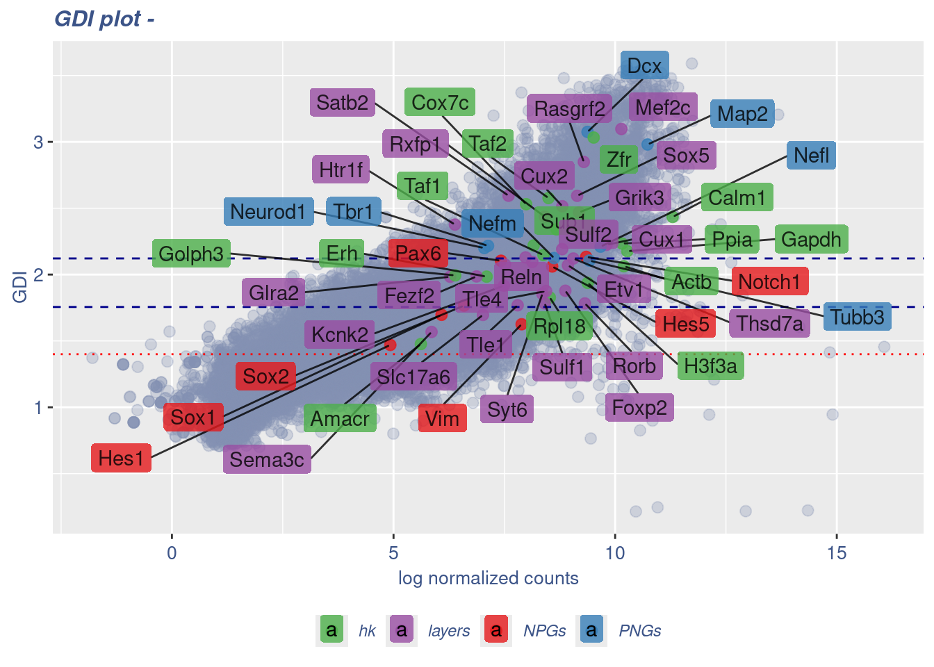
Seurat correlation
srat<- CreateSeuratObject(counts = getRawData(obj),
                          project = project,
                          min.cells = 3,
                          min.features = 200)
srat[["percent.mt"]] <- PercentageFeatureSet(srat, pattern = "^mt-")
srat <- NormalizeData(srat)
srat <- FindVariableFeatures(srat, selection.method = "vst", nfeatures = 2000)

# plot variable features with and without labels
plot1 <- VariableFeaturePlot(srat)

plot1$data$centered_variance <- scale(plot1$data$variance.standardized,
                                      center = T,scale = F)

write.csv(plot1$data,paste0("CoexData/",
                            "Variance_Seurat_genes",
                            getMetadataElement(obj,
                                               datasetTags()[["cond"]]),".csv"))

LabelPoints(plot = plot1, points = c(genesList$NPGs,genesList$PNGs,genesList$layers), repel = TRUE)
LabelPoints(plot = plot1, points = c(genesList$hk), repel = TRUE)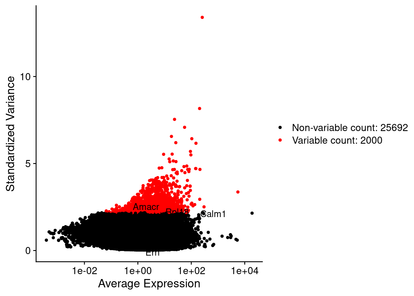
all.genes <- rownames(srat)
srat <- ScaleData(srat, features = all.genes)
seurat.data = GetAssayData(srat[["RNA"]],layer = "data")
corr.pval.list <- correlation_pvalues(data = seurat.data,
genesFromListExpressed,
n.cells = getNumCells(obj))
seurat.data.cor.big <- as.matrix(Matrix::forceSymmetric(corr.pval.list$data.cor, uplo = "U"))
htmp <- correlation_plot(seurat.data.cor.big,
genesList, title="Seurat corr")
p_values.fromSeurat <- corr.pval.list$p_values
seurat.data.cor.big <- corr.pval.list$data.cor
rm(corr.pval.list)
gc() used (Mb) gc trigger (Mb) max used (Mb)
Ncells 10214940 545.6 18206440 972.4 18206440 972.4
Vcells 433639942 3308.5 1430493239 10913.8 2772850033 21155.2draw(htmp, heatmap_legend_side="right")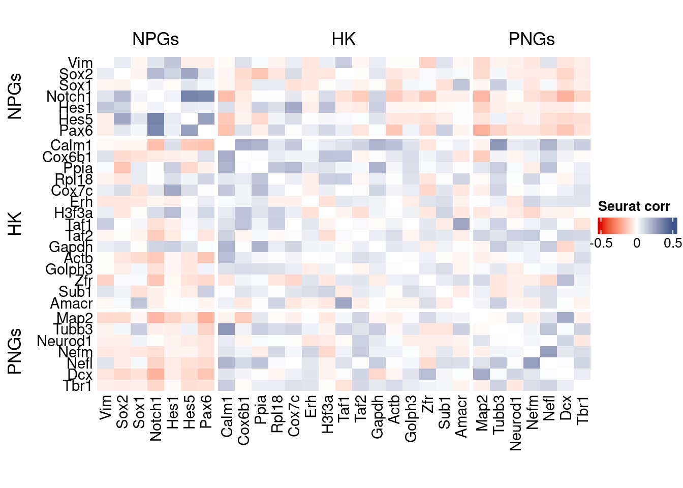
rm(seurat.data.cor.big)
rm(p_values.fromSeurat)
Seurat SC Transform
srat <-  SCTransform(srat,
                     method = "glmGamPoi",
                     vars.to.regress = "percent.mt",
                     verbose = FALSE)

seurat.data <- GetAssayData(srat[["SCT"]],layer = "data")

#Remove genes with all zeros
seurat.data <-seurat.data[rowSums(seurat.data) > 0,]


corr.pval.list <- correlation_pvalues(seurat.data,
                                      genesFromListExpressed,
                                      n.cells = getNumCells(obj))


seurat.data.cor.big <- as.matrix(Matrix::forceSymmetric(corr.pval.list$data.cor, uplo = "U"))

htmp <- correlation_plot(seurat.data.cor.big,
                         genesList, title="Seurat corr SCT")


p_values.fromSeurat <- corr.pval.list$p_values
seurat.data.cor.big <- corr.pval.list$data.cor

rm(corr.pval.list)
gc()
used (Mb) gc trigger (Mb) max used (Mb)
Ncells 10543443 563.1 18206440 972.4 18206440 972.4
Vcells 443662398 3384.9 1430493239 10913.8 2772850033 21155.2draw(htmp, heatmap_legend_side="right")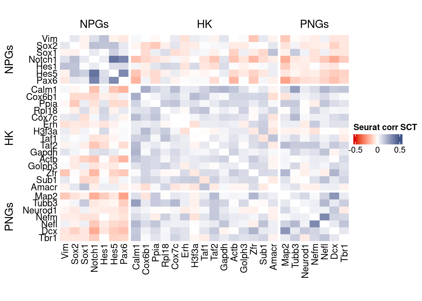
plot1 <- VariableFeaturePlot(srat)

plot1$data$centered_variance <- scale(plot1$data$residual_variance,
center = T,scale = F)write.csv(plot1$data,paste0("CoexData/",
"Variance_SeuratSCT_genes",
getMetadataElement(obj,
datasetTags()[["cond"]]),".csv"))
write_fst(as.data.frame(seurat.data.cor.big),path = paste0("CoexData/SeuratCorrSCT_",file_code,".fst"), compress = 100)
write_fst(as.data.frame(p_values.fromSeurat),path = paste0("CoexData/SeuratPValuesSCT_", file_code,".fst"))
write.csv(as.data.frame(p_values.fromSeurat),paste0("CoexData/SeuratPValuesSCT_", file_code,".csv"))
rm(seurat.data.cor.big)
rm(p_values.fromSeurat)Monocle
library(monocle3)cds <- new_cell_data_set(getRawData(obj),
cell_metadata = getMetadataCells(obj),
gene_metadata = getMetadataGenes(obj)
)
cds <- preprocess_cds(cds, num_dim = 100)
normalized_counts <- normalized_counts(cds)#Remove genes with all zeros
normalized_counts <- normalized_counts[rowSums(normalized_counts) > 0,]
corr.pval.list <- correlation_pvalues(normalized_counts,
genesFromListExpressed,
n.cells = getNumCells(obj))
rm(normalized_counts)
monocle.data.cor.big <- as.matrix(Matrix::forceSymmetric(corr.pval.list$data.cor, uplo = "U"))
htmp <- correlation_plot(data.cor.big = monocle.data.cor.big,
genesList,
title = "Monocle corr")
p_values.from.monocle <- corr.pval.list$p_values
monocle.data.cor.big <- corr.pval.list$data.cor
rm(corr.pval.list)
gc() used (Mb) gc trigger (Mb) max used (Mb)
Ncells 10729696 573.1 18206440 972.4 18206440 972.4
Vcells 446871873 3409.4 1430493239 10913.8 2772850033 21155.2draw(htmp, heatmap_legend_side="right")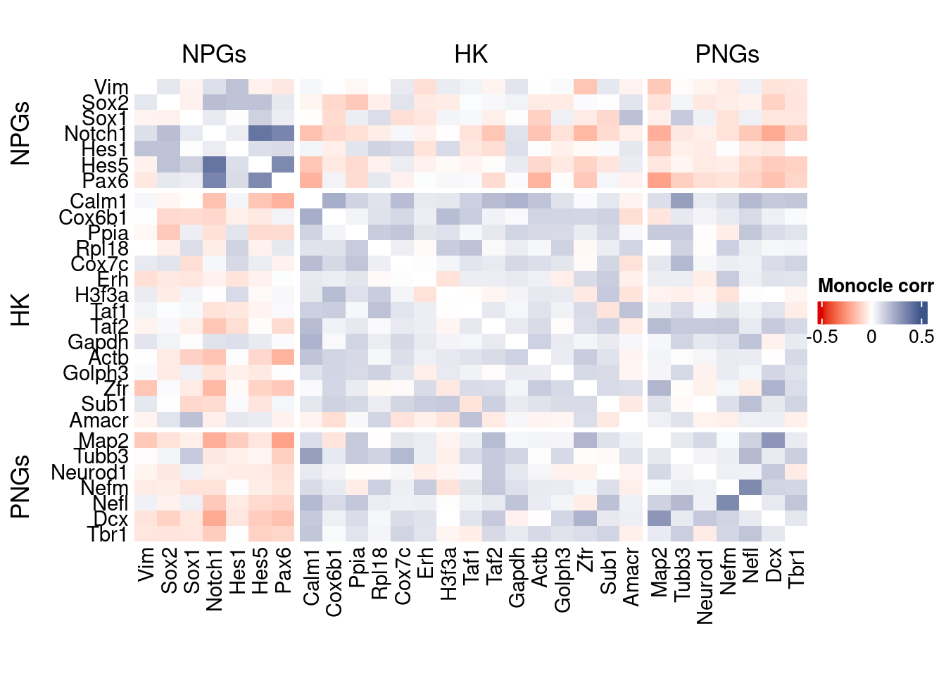
Cs-Core
library(CSCORE)Convert to Seurat obj
sceObj <- convertToSingleCellExperiment(obj)

# Correct: assay=NULL (or omit), data=NULL (since no logcounts)
seuratObj <- as.Seurat(
  x       = sceObj,
  counts  = "counts",
  data    = NULL,
  assay   = NULL,      # IMPORTANT: do NOT set to "RNA" here
  project = "COTAN"
)

# as.Seurat(SCE) creates assay "originalexp" by default; rename it to RNA
seuratObj <- RenameAssays(seuratObj, originalexp = "RNA", verbose = FALSE)
DefaultAssay(seuratObj) <- "RNA"

# Optional: keep COTAN payload
seuratObj@misc$COTAN <- S4Vectors::metadata(sceObj)
Extract CS_CORE corr matrix
seuratObj@assays$RNA@counts <- ceiling(seuratObj@assays$RNA@counts)
csCoreRes <- CSCORE(seuratObj, genes = genesFromListExpressed)
[INFO] IRLS converged after 2 iterations.
[INFO] Starting WLS for covariance at Wed Jan 21 11:38:52 2026
[INFO] 0.0649% co-expression estimates were greater than 1 and were set to 1.
[INFO] 0.0000% co-expression estimates were smaller than -1 and were set to -1.
[INFO] Finished WLS. Elapsed time: 0.0180 seconds.mat <- as.matrix(csCoreRes$est)
diag(mat) <- 0
split.genes <- base::factor(c(rep("NPGs",sum(genesList[["NPGs"]] %in% genesFromListExpressed)),
rep("HK",sum(genesList[["hk"]] %in% genesFromListExpressed)),
rep("PNGs",sum(genesList[["PNGs"]] %in% genesFromListExpressed))
),
levels = c("NPGs","HK","PNGs"))
f1 = colorRamp2(seq(-0.5,0.5, length = 3), c("#DC0000B2", "white","#3C5488B2" ))
htmp <- Heatmap(mat[c(genesList$NPGs[genesList$NPGs %in% genesFromListExpressed],genesList$hk[genesList$hk %in% genesFromListExpressed],genesList$PNGs[genesList$PNGs %in% genesFromListExpressed]),
c(genesList$NPGs[genesList$NPGs %in% genesFromListExpressed],genesList$hk[genesList$hk %in% genesFromListExpressed],genesList$PNGs[genesList$PNGs %in% genesFromListExpressed])],
#width = ncol(coexMat)*unit(2.5, "mm"),
height = nrow(mat)*unit(3, "mm"),
cluster_rows = FALSE,
cluster_columns = FALSE,
col = f1,
row_names_side = "left",
row_names_gp = gpar(fontsize = 11),
column_names_gp = gpar(fontsize = 11),
column_split = split.genes,
row_split = split.genes,
cluster_row_slices = FALSE,
cluster_column_slices = FALSE,
heatmap_legend_param = list(
title = "CS-CORE", at = c(-0.5, 0, 0.5),
direction = "horizontal",
labels = c("-0.5", "0", "0.5")
)
)
draw(htmp, heatmap_legend_side="right")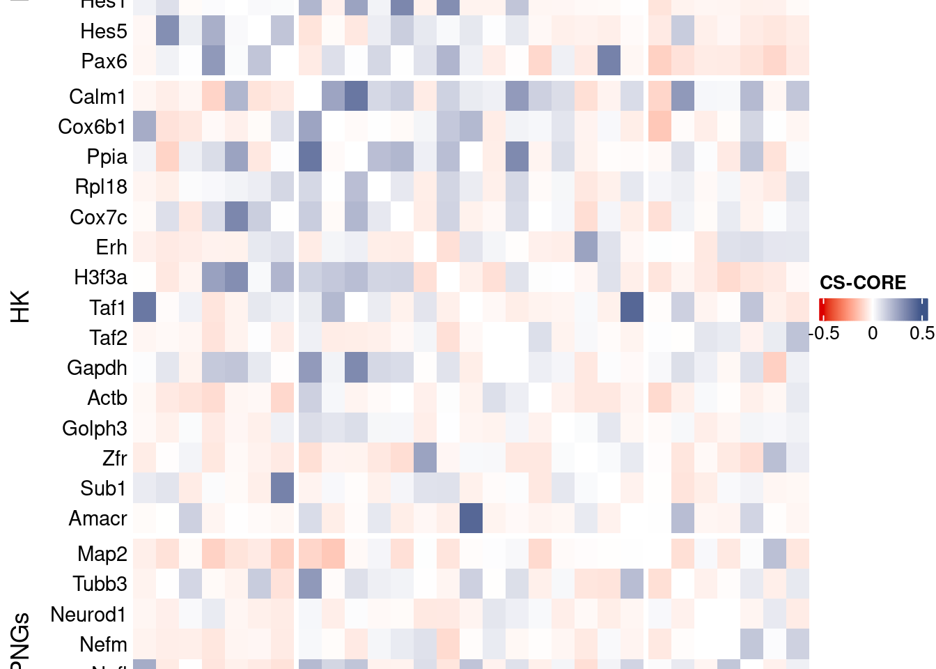
Save CS_CORE matrix
write_fst(as.data.frame(csCoreRes$est), path = paste0("CoexData/CS_CORECorr_", file_code,".fst"),compress = 100)
write_fst(as.data.frame(csCoreRes$p_value), path = paste0("CoexData/CS_COREPValues_", file_code,".fst"),compress = 100)
write.csv(as.data.frame(csCoreRes$p_value), paste0("CoexData/CS_COREPValues_", file_code,".csv"))
Baseline: Spearman on UMI counts
corr.pval.list <- correlation_pvaluesSpearman(data = getRawData(obj),
                                      genesFromListExpressed,
                                      n.cells = getNumCells(obj))

data.cor.big <- as.matrix(Matrix::forceSymmetric(corr.pval.list$data.cor, uplo = "U"))

htmp <- correlation_plot(data.cor.big,
                         genesList, title="UMI baseline S. corr")


p_values.fromSp.C <- corr.pval.list$p_values
data.cor.bigSp.C <- corr.pval.list$data.cor

rm(corr.pval.list)
gc()
used (Mb) gc trigger (Mb) max used (Mb)
Ncells 10739044 573.6 18206440 972.4 18206440 972.4
Vcells 449664836 3430.7 1430493239 10913.8 2772850033 21155.2draw(htmp, heatmap_legend_side="right")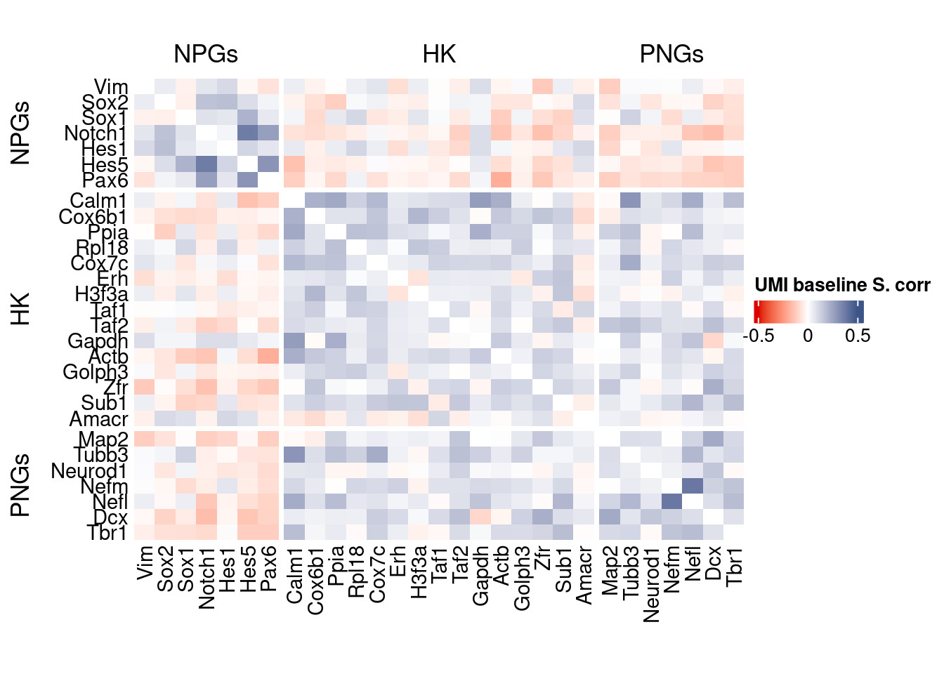
write.csv(as.data.frame(p_values.fromSp.C), paste0("CoexData/BaselineUMISpCorrPValues_", file_code,".csv"))Baseline: Pearson on binarized counts
corr.pval.list <- correlation_pvalues(data = getZeroOneProj(obj),
                                      genesFromListExpressed,
                                      n.cells = getNumCells(obj))

data.cor.big <- as.matrix(Matrix::forceSymmetric(corr.pval.list$data.cor, uplo = "U"))

htmp <- correlation_plot(data.cor.big,
                         genesList, title="Zero-one P. corr")


p_values.fromSp.C <- corr.pval.list$p_values
data.cor.bigSp.C <- corr.pval.list$data.cor

rm(corr.pval.list)
gc()
used (Mb) gc trigger (Mb) max used (Mb)
Ncells 10739171 573.6 18206440 972.4 18206440 972.4
Vcells 449665095 3430.7 1430493239 10913.8 2772850033 21155.2draw(htmp, heatmap_legend_side="right")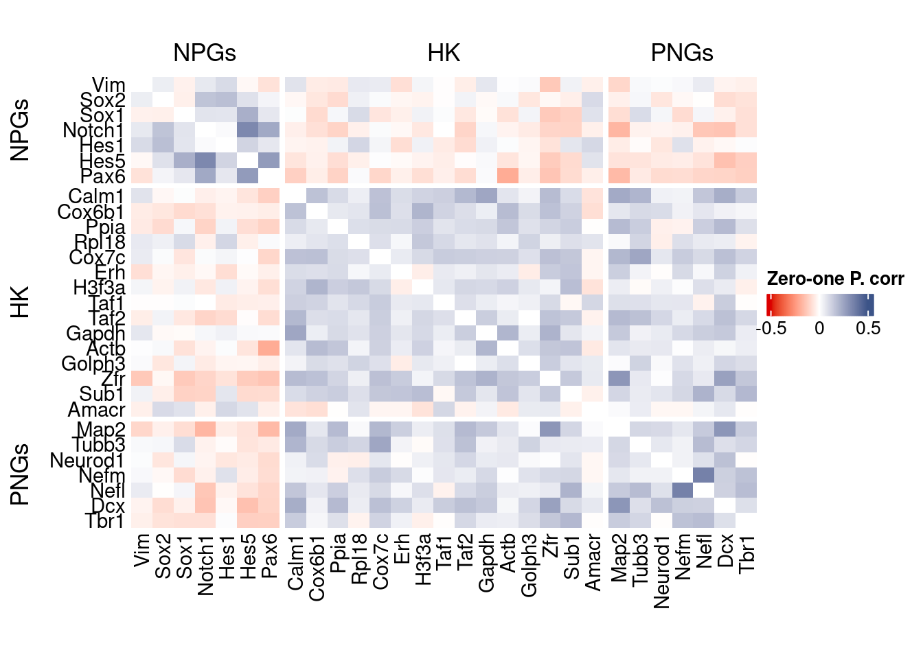
write.csv(as.data.frame(p_values.fromSp.C), paste0("CoexData/ZeroOnePCorrPValues_", file_code,".csv"))Sys.time()[1] "2026-01-21 11:38:55 CET"sessionInfo()R version 4.5.2 (2025-10-31)
Platform: x86_64-pc-linux-gnu
Running under: Ubuntu 22.04.5 LTS
Matrix products: default
BLAS: /usr/lib/x86_64-linux-gnu/blas/libblas.so.3.10.0
LAPACK: /usr/lib/x86_64-linux-gnu/lapack/liblapack.so.3.10.0 LAPACK version 3.10.0
locale:
[1] LC_CTYPE=C.UTF-8 LC_NUMERIC=C LC_TIME=C.UTF-8
[4] LC_COLLATE=C.UTF-8 LC_MONETARY=C.UTF-8 LC_MESSAGES=C.UTF-8
[7] LC_PAPER=C.UTF-8 LC_NAME=C LC_ADDRESS=C
[10] LC_TELEPHONE=C LC_MEASUREMENT=C.UTF-8 LC_IDENTIFICATION=C
time zone: Europe/Rome
tzcode source: system (glibc)
attached base packages:
[1] stats4 parallel grid stats graphics grDevices utils
[8] datasets methods base
other attached packages:
[1] CSCORE_1.0.2 monocle3_1.3.7
[3] SingleCellExperiment_1.32.0 SummarizedExperiment_1.38.1
[5] GenomicRanges_1.62.1 Seqinfo_1.0.0
[7] IRanges_2.44.0 S4Vectors_0.48.0
[9] MatrixGenerics_1.22.0 matrixStats_1.5.0
[11] Biobase_2.70.0 BiocGenerics_0.56.0
[13] generics_0.1.3 fstcore_0.10.0
[15] fst_0.9.8 stringr_1.6.0
[17] HiClimR_2.2.1 doParallel_1.0.17
[19] iterators_1.0.14 foreach_1.5.2
[21] Rfast_2.1.5.1 RcppParallel_5.1.10
[23] zigg_0.0.2 Rcpp_1.1.0
[25] patchwork_1.3.2 Seurat_5.4.0
[27] SeuratObject_5.3.0 sp_2.2-0
[29] Hmisc_5.2-3 dplyr_1.1.4
[31] circlize_0.4.16 ComplexHeatmap_2.26.0
[33] COTAN_2.11.1
loaded via a namespace (and not attached):
[1] RcppAnnoy_0.0.22 splines_4.5.2
[3] later_1.4.2 tibble_3.3.0
[5] polyclip_1.10-7 rpart_4.1.24
[7] fastDummies_1.7.5 lifecycle_1.0.4
[9] Rdpack_2.6.4 globals_0.18.0
[11] lattice_0.22-7 MASS_7.3-65
[13] backports_1.5.0 ggdist_3.3.3
[15] dendextend_1.19.0 magrittr_2.0.4
[17] plotly_4.11.0 rmarkdown_2.29
[19] yaml_2.3.10 httpuv_1.6.16
[21] otel_0.2.0 glmGamPoi_1.20.0
[23] sctransform_0.4.2 spam_2.11-1
[25] spatstat.sparse_3.1-0 reticulate_1.44.1
[27] minqa_1.2.8 cowplot_1.2.0
[29] pbapply_1.7-2 RColorBrewer_1.1-3
[31] abind_1.4-8 Rtsne_0.17
[33] purrr_1.2.0 nnet_7.3-20
[35] GenomeInfoDbData_1.2.14 ggrepel_0.9.6
[37] irlba_2.3.5.1 listenv_0.10.0
[39] spatstat.utils_3.2-1 goftest_1.2-3
[41] RSpectra_0.16-2 spatstat.random_3.4-3
[43] fitdistrplus_1.2-2 parallelly_1.46.0
[45] DelayedMatrixStats_1.30.0 ncdf4_1.24
[47] codetools_0.2-20 DelayedArray_0.36.0
[49] tidyselect_1.2.1 shape_1.4.6.1
[51] UCSC.utils_1.4.0 farver_2.1.2
[53] lme4_1.1-37 ScaledMatrix_1.16.0
[55] viridis_0.6.5 base64enc_0.1-3
[57] spatstat.explore_3.6-0 jsonlite_2.0.0
[59] GetoptLong_1.1.0 Formula_1.2-5
[61] progressr_0.18.0 ggridges_0.5.6
[63] survival_3.8-3 tools_4.5.2
[65] ica_1.0-3 glue_1.8.0
[67] gridExtra_2.3 SparseArray_1.10.8
[69] xfun_0.52 distributional_0.6.0
[71] ggthemes_5.2.0 GenomeInfoDb_1.44.0
[73] withr_3.0.2 fastmap_1.2.0
[75] boot_1.3-32 digest_0.6.37
[77] rsvd_1.0.5 parallelDist_0.2.6
[79] R6_2.6.1 mime_0.13
[81] colorspace_2.1-1 Cairo_1.7-0
[83] scattermore_1.2 tensor_1.5
[85] spatstat.data_3.1-9 tidyr_1.3.1
[87] data.table_1.18.0 httr_1.4.7
[89] htmlwidgets_1.6.4 S4Arrays_1.10.1
[91] uwot_0.2.3 pkgconfig_2.0.3
[93] gtable_0.3.6 lmtest_0.9-40
[95] S7_0.2.1 XVector_0.50.0
[97] htmltools_0.5.8.1 dotCall64_1.2
[99] clue_0.3-66 scales_1.4.0
[101] png_0.1-8 reformulas_0.4.1
[103] spatstat.univar_3.1-6 rstudioapi_0.18.0
[105] knitr_1.50 reshape2_1.4.4
[107] rjson_0.2.23 nloptr_2.2.1
[109] checkmate_2.3.2 nlme_3.1-168
[111] proxy_0.4-29 zoo_1.8-14
[113] GlobalOptions_0.1.2 KernSmooth_2.23-26
[115] miniUI_0.1.2 foreign_0.8-90
[117] pillar_1.11.1 vctrs_0.7.0
[119] RANN_2.6.2 promises_1.5.0
[121] BiocSingular_1.26.1 beachmat_2.26.0
[123] xtable_1.8-4 cluster_2.1.8.1
[125] htmlTable_2.4.3 evaluate_1.0.5
[127] magick_2.9.0 zeallot_0.2.0
[129] cli_3.6.5 compiler_4.5.2
[131] rlang_1.1.7 crayon_1.5.3
[133] future.apply_1.20.0 labeling_0.4.3
[135] plyr_1.8.9 stringi_1.8.7
[137] viridisLite_0.4.2 deldir_2.0-4
[139] BiocParallel_1.44.0 assertthat_0.2.1
[141] lazyeval_0.2.2 spatstat.geom_3.6-1
[143] Matrix_1.7-4 RcppHNSW_0.6.0
[145] sparseMatrixStats_1.20.0 future_1.69.0
[147] ggplot2_4.0.1 shiny_1.12.1
[149] rbibutils_2.3 ROCR_1.0-11
[151] igraph_2.2.1