library(COTAN)
library(ComplexHeatmap)
library(circlize)
library(dplyr)
library(Hmisc)
library(Seurat)
library(patchwork)
library(Rfast)
library(parallel)
library(doParallel)
library(HiClimR)
library(stringr)
library(fst)

options(parallelly.fork.enable = TRUE)Gene Correlation Analysis for Mouse Cortex Open Problem
Prologue
dataFile <- "Data/NewDataRevision/Ding_GSE132044_H_PBMC_M_Brain_CleanedDatasets/SplitLoomsAsCOTANObjects/mouse-brain-10XV2_Cortex1_specimen1_cell2-Cleaned.RDS"

name <- str_split(dataFile,pattern = "/",simplify = T)[5]
name <- str_remove(name,pattern = "-Cleaned.RDS")

project = name

setLoggingLevel(1)
outDir <- "CoexData/"
setLoggingFile(paste0(outDir, "Logs/",name,".log"))

obj <- readRDS(dataFile)
file_code = namesource("src/Functions.R")To compare the ability of COTAN to asses the real correlation between genes we define some pools of genes:
- Constitutive genes
- Neural progenitor genes
- Pan neuronal genes
- Some layer marker genes
genesList <- list(
  "NPGs"=
    c("Nes", "Vim", "Sox2", "Sox1", "Notch1", "Hes1", "Hes5", "Pax6"),
  "PNGs"=
    c("Map2", "Tubb3", "Neurod1", "Nefm", "Nefl", "Dcx", "Tbr1"),
  "hk"=
    c("Calm1", "Cox6b1", "Ppia", "Rpl18", "Cox7c", "Erh", "H3f3a",
      "Taf1", "Taf2", "Gapdh", "Actb", "Golph3", "Zfr", "Sub1",
      "Tars", "Amacr"),
  "layers" =
    c("Reln","Lhx5","Cux1","Satb2","Tle1","Mef2c","Rorb","Sox5","Bcl11b","Fezf2","Foxp2","Ntf3","Rasgrf2","Pvrl3", "Cux2","Slc17a6", "Sema3c","Thsd7a", "Sulf2", "Kcnk2","Grik3", "Etv1", "Tle4", "Tmem200a", "Glra2", "Etv1","Htr1f", "Sulf1","Rxfp1", "Syt6")
  # From https://www.science.org/doi/10.1126/science.aam8999
)
COTAN
genesFromListExpressed <- unlist(genesList)[unlist(genesList) %in% getGenes(obj)]
int.genes <-getGenes(obj)
coexMat.big <- getGenesCoex(obj)[genesFromListExpressed,genesFromListExpressed]
coexMat <- getGenesCoex(obj)[c(genesList$NPGs,genesList$hk,genesList$PNGs),c(genesList$NPGs,genesList$hk,genesList$PNGs)]
f1 = colorRamp2(seq(-0.5,0.5, length = 3), c("#DC0000B2", "white","#3C5488B2" ))
split.genes <- base::factor(c(rep("NPGs",length(genesList[["NPGs"]])),
rep("HK",length(genesList[["hk"]])),
rep("PNGs",length(genesList[["PNGs"]]))
),
levels = c("NPGs","HK","PNGs"))
lgd = Legend(col_fun = f1, title = "COTAN coex")
htmp <- Heatmap(as.matrix(coexMat),
#width = ncol(coexMat)*unit(2.5, "mm"),
height = nrow(coexMat)*unit(3, "mm"),
cluster_rows = FALSE,
cluster_columns = FALSE,
col = f1,
row_names_side = "left",
row_names_gp = gpar(fontsize = 11),
column_names_gp = gpar(fontsize = 11),
column_split = split.genes,
row_split = split.genes,
cluster_row_slices = FALSE,
cluster_column_slices = FALSE,
heatmap_legend_param = list(
title = "COTAN coex", at = c(-0.5, 0, 0.5),
direction = "horizontal",
labels = c("-0.5", "0", "0.5")
)
)
draw(htmp, heatmap_legend_side="right")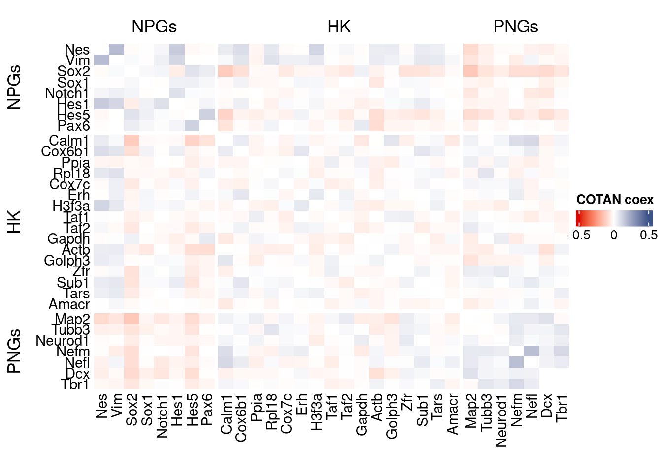
GDI_DF <- calculateGDI(obj)
GDI_DF$geneType <- NA
for (cat in names(genesList)) {
  GDI_DF[rownames(GDI_DF) %in% genesList[[cat]],]$geneType <- cat
}

GDI_DF$GDI_centered <- scale(GDI_DF$GDI,center = T,scale = T)

GDI_DF[genesFromListExpressed,]
sum.raw.norm GDI exp.cells geneType GDI_centered
Nes 2.278676 1.8853635 0.5044136 NPGs 2.409845854
Vim 4.150719 2.1708469 1.8284994 NPGs 3.521390919
Sox2 4.922471 2.0505827 3.9722573 NPGs 3.053135700
Sox1 2.090846 0.9150937 0.4413619 NPGs -1.367952638
Notch1 3.258588 1.1853252 1.1979823 NPGs -0.315791484
Hes1 5.004614 1.5276691 7.2509458 NPGs 1.017143308
Hes5 5.538588 2.1378866 6.0529634 NPGs 3.393058463
Pax6 4.521991 1.4560530 2.8373266 NPGs 0.738302140
Map2 7.216026 2.0695721 50.6935687 PNGs 3.127071898
Tubb3 5.916577 1.4126411 16.6456494 PNGs 0.569275518
Neurod1 3.694900 1.5093994 3.2786885 PNGs 0.946009059
Nefm 5.564546 1.6552262 12.5472888 PNGs 1.513793825
Nefl 5.652907 1.4733168 14.1235813 PNGs 0.805519561
Dcx 5.794682 1.5774395 18.3480454 PNGs 1.210927045
Tbr1 4.787218 1.3273611 6.4312736 PNGs 0.237232856
Calm1 7.626967 1.6533361 55.9899117 hk 1.506434412
Cox6b1 5.906675 1.4496667 17.2761665 hk 0.713436561
Ppia 4.946753 1.2920410 7.7553594 hk 0.099712361
Rpl18 4.870450 1.3869640 6.6834805 hk 0.469300252
Cox7c 5.482763 1.2909539 13.8083228 hk 0.095479551
Erh 2.885144 1.4600651 1.1979823 hk 0.753923443
H3f3a 5.660363 1.5058349 12.6733922 hk 0.932130581
Taf1 4.830185 1.2656460 8.0075662 hk -0.003058185
Taf2 5.335359 1.3987881 11.4123581 hk 0.515337873
Gapdh 3.797697 1.1165923 2.3959647 hk -0.583406636
Actb 7.982808 1.7256418 58.5119798 hk 1.787960773
Golph3 3.283765 1.2200184 1.5762926 hk -0.180711637
Zfr 6.170070 1.4428500 25.0315259 hk 0.686895385
Sub1 5.727853 1.4173439 16.4564943 hk 0.587586088
Tars 4.294292 1.2901878 4.0353090 hk 0.092496862
Amacr 3.017780 0.9962931 0.6935687 hk -1.051798341
Reln 5.156947 1.3173054 5.4854981 layers 0.198080780
Cux1 6.133925 1.4896772 19.8612863 layers 0.869219661
Satb2 5.043128 1.6840418 10.4665826 layers 1.625988650
Tle1 5.161647 1.3208315 9.1424968 layers 0.211809833
Mef2c 7.917379 2.5273429 58.6380832 layers 4.909427664
Rorb 6.368996 1.6827325 16.6456494 layers 1.620890808
Sox5 5.165735 1.3991078 9.0794451 layers 0.516582782
Bcl11b 5.909357 1.5605883 16.4564943 layers 1.145315814
Fezf2 4.739284 1.5834862 5.4854981 layers 1.234469931
Foxp2 5.662747 1.3807271 12.9255990 layers 0.445016641
Ntf3 1.854893 1.0180867 0.4413619 layers -0.966943646
Rasgrf2 4.493850 1.2256522 4.3505675 layers -0.158776080
Cux2 6.461830 1.7683723 22.6355612 layers 1.954334338
Slc17a6 3.503550 1.0962081 1.5132409 layers -0.662773626
Sema3c 4.468705 1.9659798 2.7112232 layers 2.723729856
Thsd7a 4.722444 1.2735672 5.2963430 layers 0.027783535
Sulf2 4.417151 1.2584660 4.2244641 layers -0.031013809
Kcnk2 6.536828 1.5842583 24.4640605 layers 1.237476102
Grik3 4.298769 1.2409777 3.4678436 layers -0.099105644
Etv1 5.393072 1.5012479 8.8272383 layers 0.914270724
Tle4 5.848812 1.5345867 14.1235813 layers 1.044077154
Tmem200a 3.577450 1.4204751 2.9003783 layers 0.599777545
Glra2 4.134946 1.2122619 3.2156368 layers -0.210911956
Etv1.1 5.393072 1.5012479 8.8272383 layers 0.914270724
Htr1f 5.572110 1.7947516 12.0428752 layers 2.057043339
Sulf1 3.752143 1.2018808 1.8915511 layers -0.251331258
Rxfp1 4.641643 1.3364244 4.2244641 layers 0.272521361
Syt6 4.161232 1.3292569 3.0895334 layers 0.244614598GDIPlot(obj,GDIIn = GDI_DF, genes = genesList,GDIThreshold = 1.4)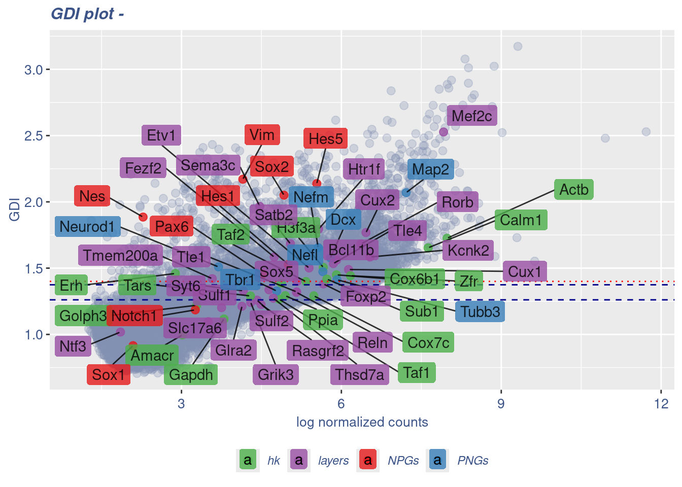
Seurat correlation
srat<- CreateSeuratObject(counts = getRawData(obj),
                          project = project,
                          min.cells = 3,
                          min.features = 200)
srat[["percent.mt"]] <- PercentageFeatureSet(srat, pattern = "^mt-")
srat <- NormalizeData(srat)
srat <- FindVariableFeatures(srat, selection.method = "vst", nfeatures = 2000)

# plot variable features with and without labels
plot1 <- VariableFeaturePlot(srat)

plot1$data$centered_variance <- scale(plot1$data$variance.standardized,
                                      center = T,scale = F)

write.csv(plot1$data,paste0("CoexData/",
                            "Variance_Seurat_genes",
                            getMetadataElement(obj,
                                               datasetTags()[["cond"]]),".csv"))

LabelPoints(plot = plot1, points = c(genesList$NPGs,genesList$PNGs,genesList$layers), repel = TRUE)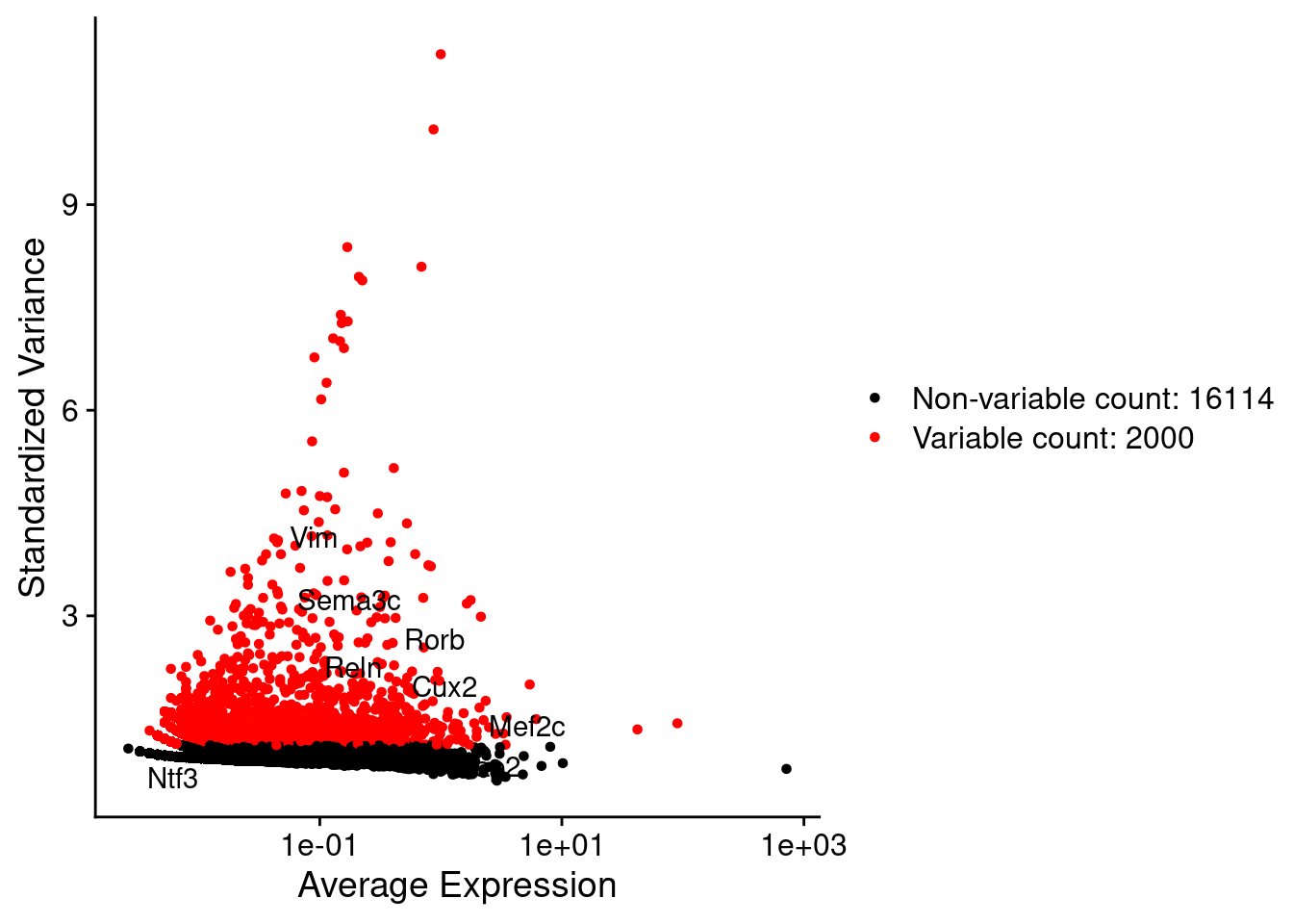
LabelPoints(plot = plot1, points = c(genesList$hk), repel = TRUE)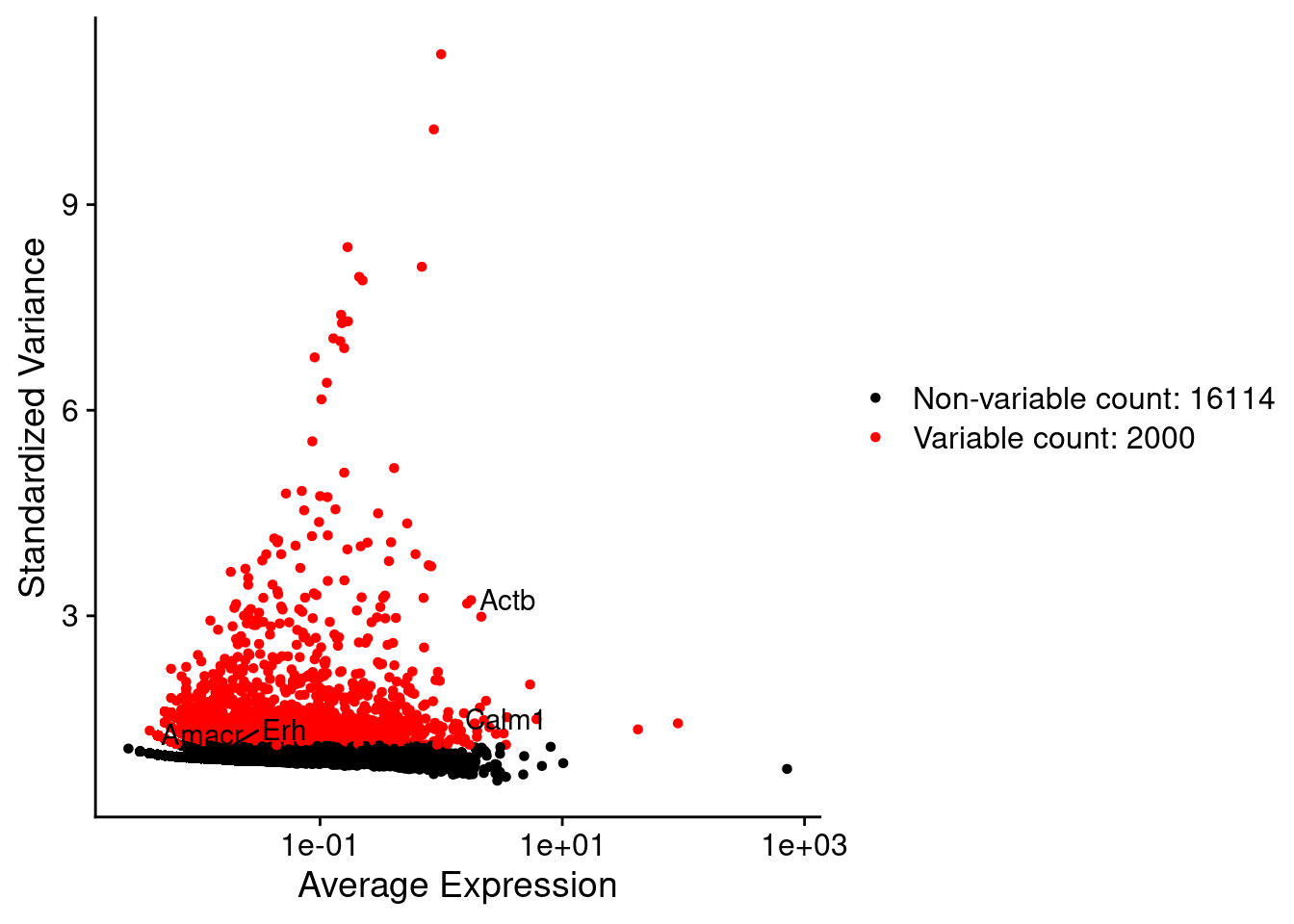
all.genes <- rownames(srat)
srat <- ScaleData(srat, features = all.genes)
seurat.data = GetAssayData(srat[["RNA"]],layer = "data")
corr.pval.list <- correlation_pvalues(data = seurat.data,
genesFromListExpressed,
n.cells = getNumCells(obj))
seurat.data.cor.big <- as.matrix(Matrix::forceSymmetric(corr.pval.list$data.cor, uplo = "U"))
htmp <- correlation_plot(seurat.data.cor.big,
genesList, title="Seurat corr")
p_values.fromSeurat <- corr.pval.list$p_values
seurat.data.cor.big <- corr.pval.list$data.cor
rm(corr.pval.list)
gc() used (Mb) gc trigger (Mb) max used (Mb)
Ncells 10170976 543.2 18206887 972.4 18206887 972.4
Vcells 222588422 1698.3 621313178 4740.3 1205067016 9194.0draw(htmp, heatmap_legend_side="right")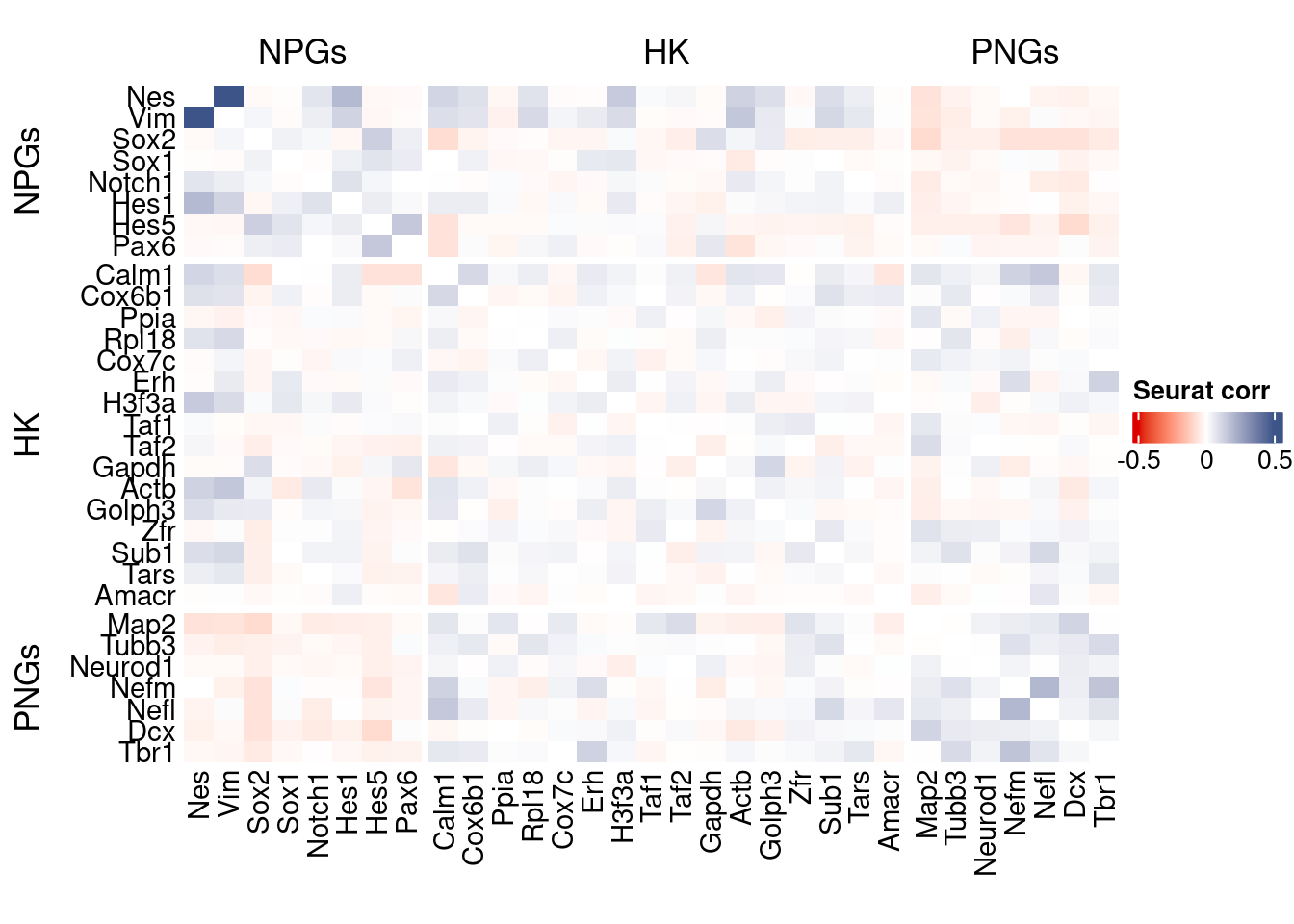
rm(seurat.data.cor.big)
rm(p_values.fromSeurat)
Seurat SC Transform
srat <-  SCTransform(srat,
                     method = "glmGamPoi",
                     vars.to.regress = "percent.mt",
                     verbose = FALSE)

seurat.data <- GetAssayData(srat[["SCT"]],layer = "data")

#Remove genes with all zeros
seurat.data <-seurat.data[rowSums(seurat.data) > 0,]


corr.pval.list <- correlation_pvalues(seurat.data,
                                      genesFromListExpressed,
                                      n.cells = getNumCells(obj))


seurat.data.cor.big <- as.matrix(Matrix::forceSymmetric(corr.pval.list$data.cor, uplo = "U"))

htmp <- correlation_plot(seurat.data.cor.big,
                         genesList, title="Seurat corr SCT")


p_values.fromSeurat <- corr.pval.list$p_values
seurat.data.cor.big <- corr.pval.list$data.cor

rm(corr.pval.list)
gc()
used (Mb) gc trigger (Mb) max used (Mb)
Ncells 10499484 560.8 18206887 972.4 18206887 972.4
Vcells 233603450 1782.3 621313178 4740.3 1205067016 9194.0draw(htmp, heatmap_legend_side="right")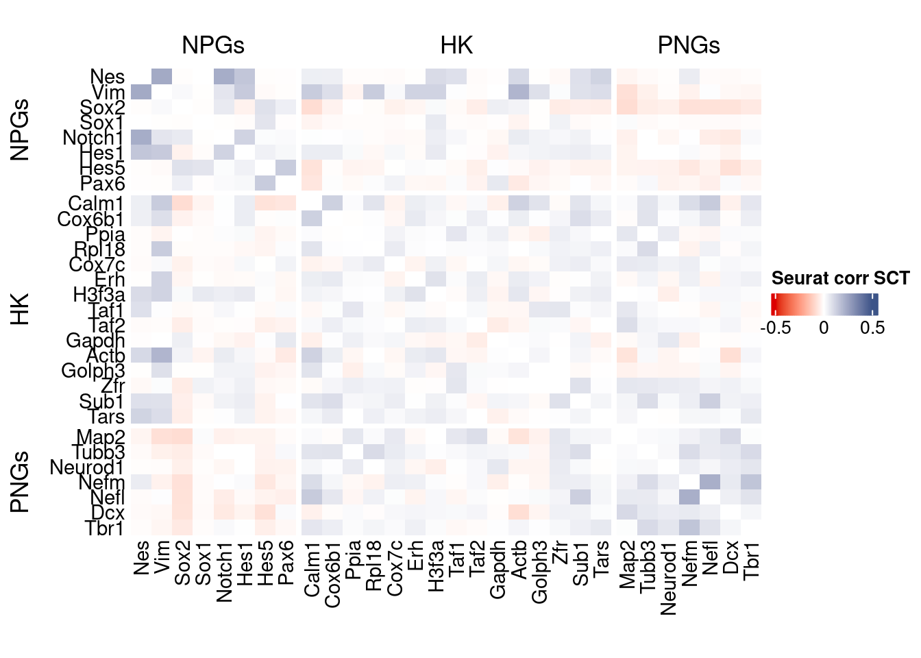
plot1 <- VariableFeaturePlot(srat)

plot1$data$centered_variance <- scale(plot1$data$residual_variance,
center = T,scale = F)write.csv(plot1$data,paste0("CoexData/",
"Variance_SeuratSCT_genes",
getMetadataElement(obj,
datasetTags()[["cond"]]),".csv"))
write_fst(as.data.frame(seurat.data.cor.big),path = paste0("CoexData/SeuratCorrSCT_",file_code,".fst"), compress = 100)
write_fst(as.data.frame(p_values.fromSeurat),path = paste0("CoexData/SeuratPValuesSCT_", file_code,".fst"))
write.csv(as.data.frame(p_values.fromSeurat),paste0("CoexData/SeuratPValuesSCT_", file_code,".csv"))
rm(seurat.data.cor.big)
rm(p_values.fromSeurat)Monocle
library(monocle3)cds <- new_cell_data_set(getRawData(obj),
cell_metadata = getMetadataCells(obj),
gene_metadata = getMetadataGenes(obj)
)
cds <- preprocess_cds(cds, num_dim = 100)
normalized_counts <- normalized_counts(cds)#Remove genes with all zeros
normalized_counts <- normalized_counts[rowSums(normalized_counts) > 0,]
corr.pval.list <- correlation_pvalues(normalized_counts,
genesFromListExpressed,
n.cells = getNumCells(obj))
rm(normalized_counts)
monocle.data.cor.big <- as.matrix(Matrix::forceSymmetric(corr.pval.list$data.cor, uplo = "U"))
htmp <- correlation_plot(data.cor.big = monocle.data.cor.big,
genesList,
title = "Monocle corr")
p_values.from.monocle <- corr.pval.list$p_values
monocle.data.cor.big <- corr.pval.list$data.cor
rm(corr.pval.list)
gc() used (Mb) gc trigger (Mb) max used (Mb)
Ncells 10685745 570.7 18206887 972.4 18206887 972.4
Vcells 235938540 1800.1 621313178 4740.3 1205067016 9194.0draw(htmp, heatmap_legend_side="right")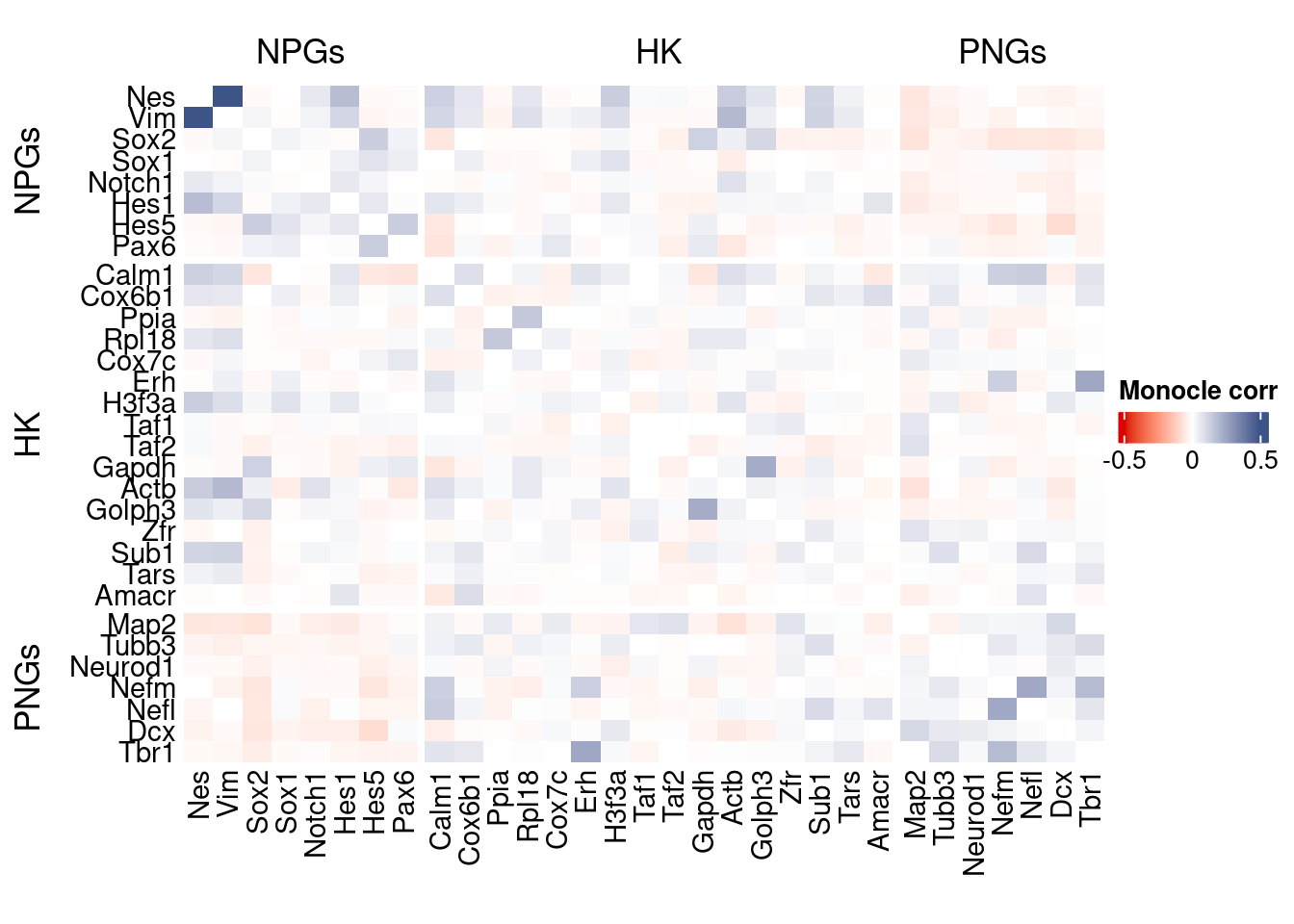
ScanPy
library(reticulate)

dirOutScP <- paste0("CoexData/ScanPy/")
if (!dir.exists(dirOutScP)) {
  dir.create(dirOutScP)
}
if(Sys.info()[["sysname"]] == "Windows"){

  use_python("C:/Users/Silvia/miniconda3/envs/r-scanpy/python.exe", required = TRUE)
  #Sys.setenv(RETICULATE_PYTHON = "C:/Users/Silvia/AppData/Local/Python/pythoncore-3.14-64/python.exe" )
}else{
  Sys.setenv(RETICULATE_PYTHON = "../../../bin/python3")
}

  py <- import("sys")

  source_python("src/scanpyGenesExpression.py")
  scanpyFDR(getRawData(obj),
                  getMetadataCells(obj),
                  getMetadataGenes(obj),
                   "mt",
                   dirOutScP,
                   file_code,
            int.genes)
inizio
open pdfnormalized_counts <- read.csv(paste0(dirOutScP,
file_code,"_Scanpy_expression_all_genes.gz"),header = T,row.names = 1)
normalized_counts <- t(normalized_counts)#Remove genes with all zeros
normalized_counts <-normalized_counts[rowSums(normalized_counts) > 0,]
corr.pval.list <- correlation_pvalues(normalized_counts,
genesFromListExpressed,
n.cells = getNumCells(obj))
ScanPy.data.cor.big <- as.matrix(Matrix::forceSymmetric(corr.pval.list$data.cor, uplo = "U"))
htmp <- correlation_plot(data.cor.big = ScanPy.data.cor.big,
genesList,
title = "ScanPy corr")
p_values.from.ScanPy <- corr.pval.list$p_values
ScanPy.data.cor.big <- corr.pval.list$data.cor
rm(corr.pval.list)
gc() used (Mb) gc trigger (Mb) max used (Mb)
Ncells 10707346 571.9 18206887 972.4 18206887 972.4
Vcells 267685109 2042.3 621313178 4740.3 1205067016 9194.0draw(htmp, heatmap_legend_side="right")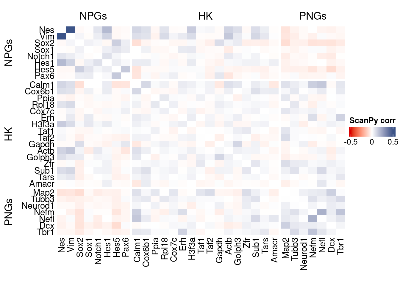
Cs-Core
library(CSCORE)Convert to Seurat obj
sceObj <- convertToSingleCellExperiment(obj)

# Correct: assay=NULL (or omit), data=NULL (since no logcounts)
seuratObj <- as.Seurat(
  x       = sceObj,
  counts  = "counts",
  data    = NULL,
  assay   = NULL,      # IMPORTANT: do NOT set to "RNA" here
  project = "COTAN"
)

# as.Seurat(SCE) creates assay "originalexp" by default; rename it to RNA
seuratObj <- RenameAssays(seuratObj, originalexp = "RNA", verbose = FALSE)
DefaultAssay(seuratObj) <- "RNA"

# Optional: keep COTAN payload
seuratObj@misc$COTAN <- S4Vectors::metadata(sceObj)
Extract CS_CORE corr matrix
#seuratObj@assays$RNA@counts <- ceiling(seuratObj@assays$RNA@counts)
csCoreRes <- CSCORE(seuratObj, genes = genesFromListExpressed)
[INFO] IRLS converged after 3 iterations.
[INFO] Starting WLS for covariance at Fri Jan 23 10:55:50 2026
[INFO] 7 among 59 genes have invalid variance estimates. Their co-expressions with other genes were set to 0.
[INFO] 1.4027% co-expression estimates were greater than 1 and were set to 1.
[INFO] 1.8703% co-expression estimates were smaller than -1 and were set to -1.
[INFO] Finished WLS. Elapsed time: 0.0487 seconds.mat <- as.matrix(csCoreRes$est)
diag(mat) <- 0
split.genes <- base::factor(c(rep("NPGs",sum(genesList[["NPGs"]] %in% genesFromListExpressed)),
rep("HK",sum(genesList[["hk"]] %in% genesFromListExpressed)),
rep("PNGs",sum(genesList[["PNGs"]] %in% genesFromListExpressed))
),
levels = c("NPGs","HK","PNGs"))
f1 = colorRamp2(seq(-0.5,0.5, length = 3), c("#DC0000B2", "white","#3C5488B2" ))
htmp <- Heatmap(as.matrix(mat[c(genesList$NPGs,genesList$hk,genesList$PNGs),c(genesList$NPGs,genesList$hk,genesList$PNGs)]),
#width = ncol(coexMat)*unit(2.5, "mm"),
height = nrow(mat)*unit(3, "mm"),
cluster_rows = FALSE,
cluster_columns = FALSE,
col = f1,
row_names_side = "left",
row_names_gp = gpar(fontsize = 11),
column_names_gp = gpar(fontsize = 11),
column_split = split.genes,
row_split = split.genes,
cluster_row_slices = FALSE,
cluster_column_slices = FALSE,
heatmap_legend_param = list(
title = "CS-CORE", at = c(-0.5, 0, 0.5),
direction = "horizontal",
labels = c("-0.5", "0", "0.5")
)
)
draw(htmp, heatmap_legend_side="right")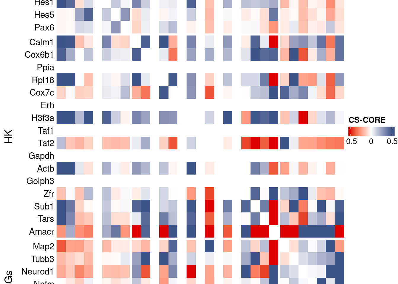
Save CS_CORE matrix
write_fst(as.data.frame(csCoreRes$est), path = paste0("CoexData/CS_CORECorr_", file_code,".fst"),compress = 100)
write_fst(as.data.frame(csCoreRes$p_value), path = paste0("CoexData/CS_COREPValues_", file_code,".fst"),compress = 100)
write.csv(as.data.frame(csCoreRes$p_value), paste0("CoexData/CS_COREPValues_", file_code,".csv"))
Baseline: Spearman on UMI counts
corr.pval.list <- correlation_pvaluesSpearman(data = getRawData(obj),
                                      genesFromListExpressed,
                                      n.cells = getNumCells(obj))

data.cor.big <- as.matrix(Matrix::forceSymmetric(corr.pval.list$data.cor, uplo = "U"))

htmp <- correlation_plot(data.cor.big,
                         genesList, title="UMI baseline S. corr")


p_values.fromSp.C <- corr.pval.list$p_values
data.cor.bigSp.C <- corr.pval.list$data.cor

rm(corr.pval.list)
gc()
used (Mb) gc trigger (Mb) max used (Mb)
Ncells 10715628 572.3 18206887 972.4 18206887 972.4
Vcells 265408044 2025.0 621313178 4740.3 1205067016 9194.0draw(htmp, heatmap_legend_side="right")
write.csv(as.data.frame(p_values.fromSp.C), paste0("CoexData/BaselineUMISpCorrPValues_", file_code,".csv"))Baseline: Pearson on binarized counts
corr.pval.list <- correlation_pvalues(data = getZeroOneProj(obj),
                                      genesFromListExpressed,
                                      n.cells = getNumCells(obj))

data.cor.big <- as.matrix(Matrix::forceSymmetric(corr.pval.list$data.cor, uplo = "U"))

htmp <- correlation_plot(data.cor.big,
                         genesList, title="Zero-one P. corr")


p_values.fromSp.C <- corr.pval.list$p_values
data.cor.bigSp.C <- corr.pval.list$data.cor

rm(corr.pval.list)
gc()
used (Mb) gc trigger (Mb) max used (Mb)
Ncells 10715800 572.3 18206887 972.4 18206887 972.4
Vcells 265408381 2025.0 621313178 4740.3 1205067016 9194.0draw(htmp, heatmap_legend_side="right")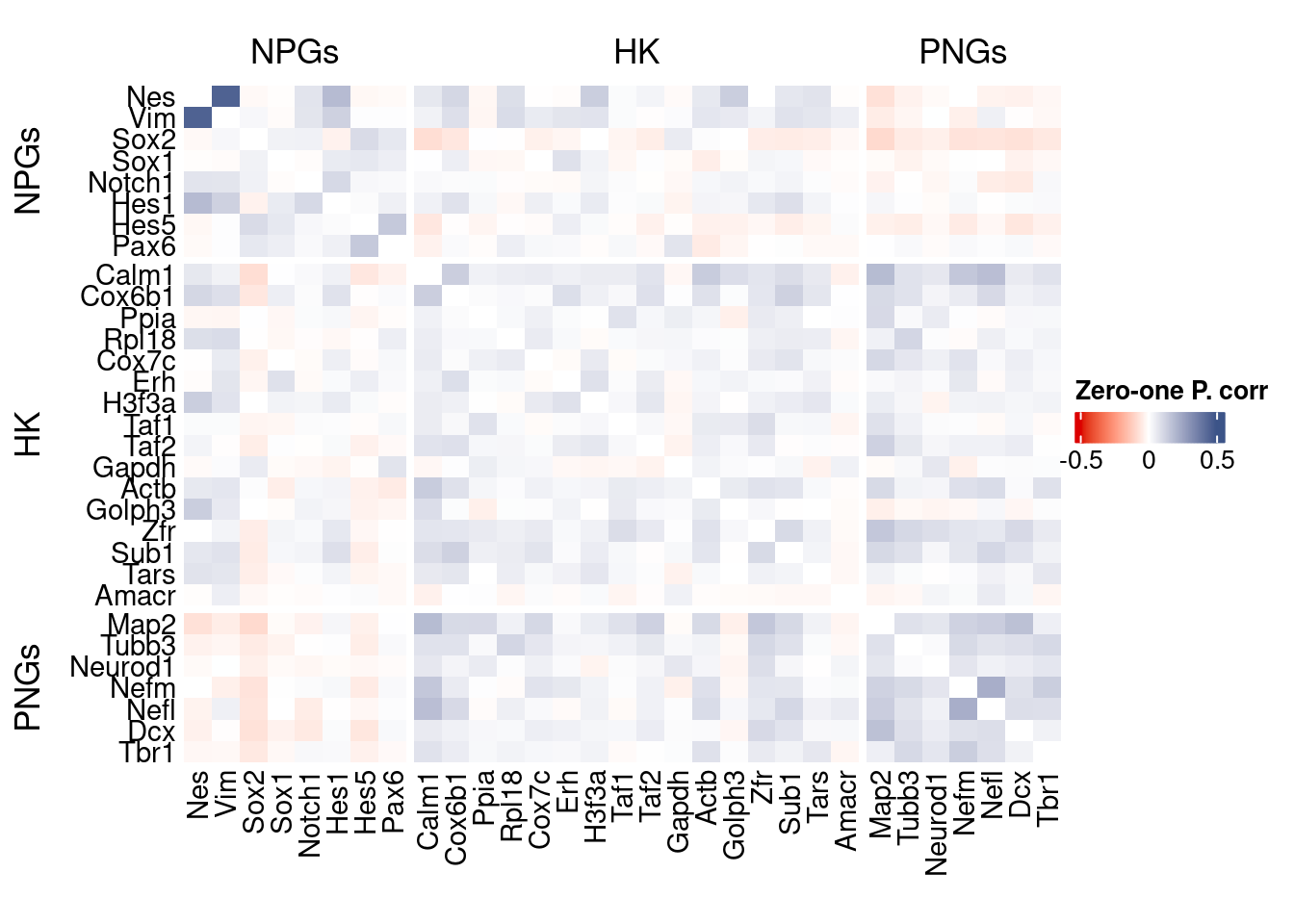
write.csv(as.data.frame(p_values.fromSp.C), paste0("CoexData/ZeroOnePCorrPValues_", file_code,".csv"))Sys.time()[1] "2026-01-23 10:55:55 CET"sessionInfo()R version 4.5.2 (2025-10-31)
Platform: x86_64-pc-linux-gnu
Running under: Ubuntu 22.04.5 LTS
Matrix products: default
BLAS: /usr/lib/x86_64-linux-gnu/blas/libblas.so.3.10.0
LAPACK: /usr/lib/x86_64-linux-gnu/lapack/liblapack.so.3.10.0 LAPACK version 3.10.0
locale:
[1] LC_CTYPE=C.UTF-8 LC_NUMERIC=C LC_TIME=C.UTF-8
[4] LC_COLLATE=C.UTF-8 LC_MONETARY=C.UTF-8 LC_MESSAGES=C.UTF-8
[7] LC_PAPER=C.UTF-8 LC_NAME=C LC_ADDRESS=C
[10] LC_TELEPHONE=C LC_MEASUREMENT=C.UTF-8 LC_IDENTIFICATION=C
time zone: Europe/Rome
tzcode source: system (glibc)
attached base packages:
[1] stats4 parallel grid stats graphics grDevices utils
[8] datasets methods base
other attached packages:
[1] CSCORE_1.0.2 reticulate_1.44.1
[3] monocle3_1.3.7 SingleCellExperiment_1.32.0
[5] SummarizedExperiment_1.38.1 GenomicRanges_1.62.1
[7] Seqinfo_1.0.0 IRanges_2.44.0
[9] S4Vectors_0.48.0 MatrixGenerics_1.22.0
[11] matrixStats_1.5.0 Biobase_2.70.0
[13] BiocGenerics_0.56.0 generics_0.1.3
[15] fstcore_0.10.0 fst_0.9.8
[17] stringr_1.6.0 HiClimR_2.2.1
[19] doParallel_1.0.17 iterators_1.0.14
[21] foreach_1.5.2 Rfast_2.1.5.1
[23] RcppParallel_5.1.10 zigg_0.0.2
[25] Rcpp_1.1.0 patchwork_1.3.2
[27] Seurat_5.4.0 SeuratObject_5.3.0
[29] sp_2.2-0 Hmisc_5.2-3
[31] dplyr_1.1.4 circlize_0.4.16
[33] ComplexHeatmap_2.26.0 COTAN_2.11.1
loaded via a namespace (and not attached):
[1] RcppAnnoy_0.0.22 splines_4.5.2
[3] later_1.4.2 tibble_3.3.0
[5] polyclip_1.10-7 rpart_4.1.24
[7] fastDummies_1.7.5 lifecycle_1.0.4
[9] Rdpack_2.6.4 globals_0.18.0
[11] lattice_0.22-7 MASS_7.3-65
[13] backports_1.5.0 ggdist_3.3.3
[15] dendextend_1.19.0 magrittr_2.0.4
[17] plotly_4.11.0 rmarkdown_2.29
[19] yaml_2.3.10 httpuv_1.6.16
[21] otel_0.2.0 glmGamPoi_1.20.0
[23] sctransform_0.4.2 spam_2.11-1
[25] spatstat.sparse_3.1-0 minqa_1.2.8
[27] cowplot_1.2.0 pbapply_1.7-2
[29] RColorBrewer_1.1-3 abind_1.4-8
[31] Rtsne_0.17 purrr_1.2.0
[33] nnet_7.3-20 GenomeInfoDbData_1.2.14
[35] ggrepel_0.9.6 irlba_2.3.5.1
[37] listenv_0.10.0 spatstat.utils_3.2-1
[39] goftest_1.2-3 RSpectra_0.16-2
[41] spatstat.random_3.4-3 fitdistrplus_1.2-2
[43] parallelly_1.46.0 DelayedMatrixStats_1.30.0
[45] ncdf4_1.24 codetools_0.2-20
[47] DelayedArray_0.36.0 tidyselect_1.2.1
[49] shape_1.4.6.1 UCSC.utils_1.4.0
[51] farver_2.1.2 lme4_1.1-37
[53] ScaledMatrix_1.16.0 viridis_0.6.5
[55] base64enc_0.1-3 spatstat.explore_3.6-0
[57] jsonlite_2.0.0 GetoptLong_1.1.0
[59] Formula_1.2-5 progressr_0.18.0
[61] ggridges_0.5.6 survival_3.8-3
[63] tools_4.5.2 ica_1.0-3
[65] glue_1.8.0 gridExtra_2.3
[67] SparseArray_1.10.8 xfun_0.52
[69] distributional_0.6.0 ggthemes_5.2.0
[71] GenomeInfoDb_1.44.0 withr_3.0.2
[73] fastmap_1.2.0 boot_1.3-32
[75] digest_0.6.37 rsvd_1.0.5
[77] parallelDist_0.2.6 R6_2.6.1
[79] mime_0.13 colorspace_2.1-1
[81] Cairo_1.7-0 scattermore_1.2
[83] tensor_1.5 spatstat.data_3.1-9
[85] tidyr_1.3.1 data.table_1.18.0
[87] httr_1.4.7 htmlwidgets_1.6.4
[89] S4Arrays_1.10.1 uwot_0.2.3
[91] pkgconfig_2.0.3 gtable_0.3.6
[93] lmtest_0.9-40 S7_0.2.1
[95] XVector_0.50.0 htmltools_0.5.8.1
[97] dotCall64_1.2 clue_0.3-66
[99] scales_1.4.0 png_0.1-8
[101] reformulas_0.4.1 spatstat.univar_3.1-6
[103] rstudioapi_0.18.0 knitr_1.50
[105] reshape2_1.4.4 rjson_0.2.23
[107] nloptr_2.2.1 checkmate_2.3.2
[109] nlme_3.1-168 proxy_0.4-29
[111] zoo_1.8-14 GlobalOptions_0.1.2
[113] KernSmooth_2.23-26 miniUI_0.1.2
[115] foreign_0.8-90 pillar_1.11.1
[117] vctrs_0.7.0 RANN_2.6.2
[119] promises_1.5.0 BiocSingular_1.26.1
[121] beachmat_2.26.0 xtable_1.8-4
[123] cluster_2.1.8.1 htmlTable_2.4.3
[125] evaluate_1.0.5 magick_2.9.0
[127] zeallot_0.2.0 cli_3.6.5
[129] compiler_4.5.2 rlang_1.1.7
[131] crayon_1.5.3 future.apply_1.20.0
[133] labeling_0.4.3 plyr_1.8.9
[135] stringi_1.8.7 viridisLite_0.4.2
[137] deldir_2.0-4 BiocParallel_1.44.0
[139] assertthat_0.2.1 lazyeval_0.2.2
[141] spatstat.geom_3.6-1 Matrix_1.7-4
[143] RcppHNSW_0.6.0 sparseMatrixStats_1.20.0
[145] future_1.69.0 ggplot2_4.0.1
[147] shiny_1.12.1 rbibutils_2.3
[149] ROCR_1.0-11 igraph_2.2.1